


BER (Bit Error Rate) counts wrong bits. MER (Modulation Error Ratio) measures how far your constellation points have drifted from where they should be. Together, they are the two most important quality metrics in any QAM-based digital transmission system — from cable TV headends to satellite downlinks to FTTH PONs. This guide gives you the definitions, the formulas, the real-world thresholds, and the engineering context you need to use both metrics correctly.
1. Why BER and MER Matter
Every digital transmission system has one job: deliver bits from point A to point B without errors. In practice, noise, distortion, and impairments corrupt the signal. The question is always the same — how much corruption is too much?
Two metrics answer that question from different angles:
| Metric | What It Measures | Units | Typical Range |
|---|---|---|---|
| BER | Ratio of errored bits to total transmitted bits | Dimensionless (10−x) | 10−3 to 10−12 |
| MER | Ratio of ideal signal power to error-vector power | dB | 15 dB to 40+ dB |
BER is a result metric — it tells you the outcome after all impairments have done their damage. MER is a process metric — it tells you how much margin you have before that damage becomes catastrophic. Understanding both, and the relationship between them, is essential for anyone designing, deploying, or troubleshooting digital transmission systems.
2. BER (Bit Error Rate): Definition and Formula
2.1 Definition
Bit Error Rate (BER) is the ratio of incorrectly received bits to the total number of transmitted bits over a given observation interval. It is the most fundamental measure of digital link quality.
“BER is a measure of the number of bits received in error, specifically, the number of errored bits divided by the total number of transmitted bits.” — CableLabs, DOCSIS Radio Frequency Interface Specification
2.2 Formula
Where:
- = number of errored bits
- = total number of transmitted bits
BER is typically expressed in scientific notation as 10−x. For example:
- BER = 10−9 → on average, 1 bit error per 1,000,000,000 bits transmitted
- BER = 10−6 → on average, 1 bit error per 1,000,000 bits transmitted
- BER = 10−3 → 1 error per 1,000 bits (unacceptable for most systems)
2.3 Industry-Standard BER Thresholds
Different applications tolerate different BER levels. The following are well-established targets from ITU-T and cable industry standards:
| Application | Target BER | Standard Reference |
|---|---|---|
| Cable TV (QAM, post-FEC) | 10−8 to 10−11 | ITU-T J.83 |
| Satellite DVB-S2 (post-FEC) | 10−7 to 10−11 | ETSI EN 302 307 |
| Fiber optic (ITU-T G.652) | 10−12 (per span) | ITU-T G.957 |
| LTE/5G (data channel) | 10−5 (pre-FEC) | 3GPP TS 36.211 |
| DOCSIS 3.1 (post-FEC) | 10−8 | CableLabs CM-SP-PHYv3.1 |
A BER of 10−9 is often called the “QoS threshold” in cable systems — below this, subscribers see no visible artifacts. Above 10−6, picture quality degrades noticeably; above 10−3, the link is effectively broken.
3. MER (Modulation Error Ratio): Definition and Formula
3.1 Definition
Modulation Error Ratio (MER) is the ratio of the average power of the ideal constellation symbol to the average power of the error vector, expressed in decibels. It quantifies the aggregate impact of all impairments — noise, phase noise, amplitude imbalances, compression, and inter-symbol interference — on a modulated carrier.
“MER is to QAM signals what CNR is to analog signals — a single-number summary of signal quality, but one that captures both noise and distortion.”
3.2 Formula
Where:
- = ideal (reference) in-phase and quadrature coordinates of the j-th symbol
- = error vector components (difference between received and ideal symbol position)
- = total number of symbols measured
In the constellation diagram, this translates to:
- Numerator → Average Symbol Magnitude (the distance from origin to the ideal symbol point)
- Denominator → RMS Error Magnitude (the scatter of received symbols around their ideal positions)
3.3 MER vs. CNR: A Critical Distinction
| Aspect | CNR | MER |
|---|---|---|
| What it captures | Noise only | Noise + distortion + all impairments |
| Measurement domain | RF spectrum (power in carrier vs. noise floor) | Constellation (symbol deviations) |
| Applicable to | Any carrier (analog or digital) | QAM / QPSK modulated signals only |
| Typical relationship | MER ≤ CNR | MER is always less than or equal to CNR |
MER is always ≤ CNR because CNR measures only additive noise, while MER includes noise plus all distortion products. A system with excellent CNR but poor MER likely suffers from non-linear distortion (compression, intermodulation) or phase noise — problems CNR alone cannot detect.
3.4 MER Minimum Thresholds (Post-FEC Operational)
These are widely accepted minimum MER values for error-free reception in cable networks:
| Modulation | Minimum MER (dB) | Recommended MER (dB) | Source |
|---|---|---|---|
| QPSK | ~8–10 dB | ≥ 12 dB | ETSI TR 101 290 |
| 16-QAM | ~15–16 dB | ≥ 20 dB | ITU-T J.83 |
| 64-QAM | ~23–24 dB | ≥ 28 dB | CableLabs DOCSIS |
| 256-QAM | ~28–30 dB | ≥ 34 dB | SCTE 40 |
| 1024-QAM | ~34–36 dB | ≥ 40 dB | DOCSIS 3.1 |
| 4096-QAM | ~40–42 dB | ≥ 46 dB | DOCSIS 3.1 (full spectrum) |
Below the minimum MER, the decoder enters the “cliff effect” — signal quality drops off sharply rather than degrading gracefully. A 1–2 dB drop in MER near the threshold can mean the difference between perfect reception and total failure.
4. CNR and Its Relationship to BER
4.1 The Fundamental Trade-off: Modulation Order vs. Noise Tolerance
Higher-order QAM modulation (e.g., 256-QAM vs. QPSK) increases data throughput because each symbol carries more bits. However, this comes at a cost: the amplitude levels are spaced more closely together, making them more susceptible to noise.
| Modulation | Bits per Symbol | Relative Amplitude Spacing | CNR Sensitivity |
|---|---|---|---|
| QPSK | 2 | Widest | Lowest |
| 16-QAM | 4 | Wide | Low |
| 64-QAM | 6 | Moderate | Moderate |
| 256-QAM | 8 | Narrow | High |
| 1024-QAM | 10 | Very narrow | Very high |
| 4096-QAM | 12 | Extremely narrow | Extremely high |
4.2 CNR vs. BER: The Curves
The relationship between CNR and BER follows a characteristic family of “waterfall curves” — one for each modulation order. Based on the well-established theoretical and measured data consistent with ITU-T and CableLabs references:
Approximate CNR required for BER = 10−4 (pre-FEC):
| Modulation | Required CNR (dB) |
|---|---|
| QPSK | ~5–6 dB |
| 16-QAM | ~10–11 dB |
| 64-QAM | ~16–17 dB |
| 256-QAM | ~22–23 dB |
Approximate CNR required for BER = 10−9 (near post-FEC QoS):
| Modulation | Required CNR (dB) |
|---|---|
| QPSK | ~9–10 dB |
| 16-QAM | ~14–15 dB |
| 64-QAM | ~21–22 dB |
| 256-QAM | ~27–28 dB |
Each doubling of the modulation order (in terms of bits per symbol) typically requires approximately 5–6 dB more CNR to maintain the same BER. This is one of the most important design rules in digital transmission engineering.
4.3 Practical Implication
If your 64-QAM channel measures CNR = 25 dB, you have roughly 3–4 dB of margin above the 10−9 threshold. If you upgrade to 256-QAM to gain 33% more throughput, you need at least 28 dB CNR — meaning your margin drops to zero or negative. Without improving the link budget, the upgrade will fail.
💡 Optical Link Budget Matters
When the RF-to-optical conversion in the headend introduces additional noise or distortion, the CNR delivered to the receiver is degraded before the signal even reaches the coaxial distribution plant. This is why optical transmitter quality and EDFA noise figure are critical — every dB of noise added in the optical domain directly reduces the CNR available at the receiver. A low-noise optical transmitter with NPR ≥ 52 dB preserves your CNR budget and makes higher-order QAM upgrades feasible.
5. FEC (Forward Error Correction): The Safety Net
5.1 Definition
Forward Error Correction (FEC) is a technique that adds redundant bits to the transmitted data stream so that the receiver can detect and correct bit errors without requiring retransmission.
“FEC is a procedural technique used to identify and correct bit errors occurring in digital transmission. It is complex and processor-intensive, but essential for preventing bit errors that cannot be entirely eliminated from resulting in erroneous data or degraded picture quality.”
5.2 How FEC Works
FEC encoders add parity/check bits to the payload before transmission. Common FEC schemes in cable and satellite:
| System | FEC Code | Code Rate | Correction Capability |
|---|---|---|---|
| DVB-C (ITU-T J.83A/C) | Reed-Solomon (204, 188) | ~0.92 | Up to 8 byte errors per RS block |
| DOCSIS 1.0–3.0 | Reed-Solomon + interleaver | Variable | Corrects burst errors up to ~70 µs |
| DVB-S2 | LDPC + BCH | 1/4 to 9/10 | Near-Shannon-limit performance |
| DOCSIS 3.1 | LDPC + BCH | Variable | Operates within 0.8 dB of Shannon limit |
5.3 Pre-FEC BER vs. Post-FEC BER
This distinction is critical:
- Pre-FEC BER (also called “correctable BER”): The raw error rate before FEC decoding. Values like 10−4 to 10−6 are common and expected.
- Post-FEC BER (also called “uncorrectable BER”): The residual error rate after FEC decoding. For acceptable QoS, this should be essentially zero (better than 10−11).
If post-FEC BER is non-zero, it means the FEC has been overwhelmed — the incoming error rate exceeds its correction capacity. This is a red alert condition. In cable systems, a non-zero post-FEC BER directly correlates with visible pixelation, freezing, or audio dropouts.
5.4 Coding Gain
FEC provides a coding gain — the reduction in required CNR to achieve the same post-FEC BER:
| FEC Scheme | Typical Coding Gain (dB) |
|---|---|
| Reed-Solomon (204, 188) | ~2–3 dB |
| Concatenated RS + convolutional | ~5–6 dB |
| LDPC (DVB-S2) | ~8–10 dB |
| LDPC + BCH (DOCSIS 3.1) | ~9–11 dB |
This coding gain is not “free” — it costs bandwidth. A code rate of 3/4 means 25% of the transmitted bits are overhead. But in most real-world systems, the 6–10 dB coding gain is worth far more than the bandwidth penalty.
6. NPR (Noise Power Ratio): Testing Wideband QAM Systems
6.1 Definition
Noise Power Ratio (NPR) is a measurement technique used to determine the signal-to-noise performance of analog devices — amplifiers, optical transmitters, EDFAs, and EYDFAs — when loaded with multiple QAM or QPSK carriers.
Because the combined spectrum of many QAM signals closely resembles Gaussian noise, NPR testing substitutes a broadband noise source for the actual QAM signals. A narrow notch (typically 4 MHz wide) is cut into the noise, and the depth of that notch after passing through the device under test indicates the noise and distortion contributed by the device.
“NPR is sometimes referred to as a ‘notch noise test.'”
6.2 The NPR Curve
The characteristic NPR curve reveals three distinct operating regions:
| Region | Drive Level | Behavior | Dominant Mechanism |
|---|---|---|---|
| 1. System noise limited | Low | Notch depth increases 1 dB per 1 dB increase in drive | Thermal noise, shot noise dominate |
| 2. Linear operating region | Medium | Peak NPR — maximum dynamic range | Best balance: signal above noise floor, below compression |
| 3. Compression limited | High | Notch depth decreases ~5 dB per 1 dB increase in drive | Noise-like intermodulation distortion fills the notch |
The peak of the NPR curve represents the optimal operating point — the drive level at which the device delivers the best possible CNR to the loaded QAM signals.
6.3 Practical NPR Targets
For cable distribution amplifiers and optical transmission equipment carrying 64-QAM and 256-QAM:
| Device Type | Typical Peak NPR (dB) |
|---|---|
| Push-pull amplifier | 38–42 dB |
| Power-doubling amplifier | 42–46 dB |
| GaAs hybrid amplifier | 44–48 dB |
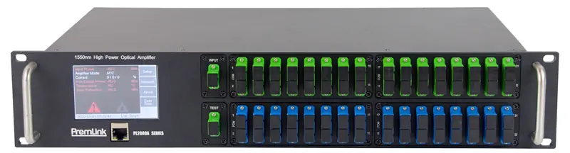
| 1550 nm optical transmitter | 50–55 dB |
| EDFA (Er-Doped Fiber Amplifier) | 52–58 dB |
| EYDFA (Er/Yb-Doped Fiber Amplifier) | 50–55 dB |
🔧 Product Spotlight: Optical Transmitters and Amplifiers for QAM Distribution
When qualifying an optical transmitter, EDFA, or EYDFA for QAM-loaded cable or FTTH distribution, NPR is the single most important specification. Here is what to look for:
- Optical Transmitter: NPR ≥ 52 dB at rated optical output. This ensures the transmitter’s noise and distortion contribution is at least 20 dB below the QAM signal level, preserving MER for 256-QAM and beyond.
- EDFA: Noise figure ≤ 5.0 dB; NPR ≥ 54 dB at operating gain. Low NF is critical because EDFA noise is additive — once added, it cannot be removed downstream. For cascaded EDFA architectures, each stage’s NF directly subtracts from the system CNR budget.
- EYDFA: For extended-reach applications requiring output power up to 27 dBm, choose EYDFA with NF ≤ 5.5 dB and NPR ≥ 50 dB. EYDFA’s higher output power enables longer spans, but the slightly higher NF means it should be placed after a pre-amplifier EDFA in the link, not as the first amplifier stage.
Rule of thumb: in a headend-to-node optical link, the combined NPR of the optical transmitter + EDFA chain must exceed the end-of-line MER requirement by at least 6 dB to account for coaxial distribution losses.
An NPR below 30 dB at the operating point means the device is adding too much noise and distortion for reliable 256-QAM operation.
7. The Cliff Effect: Why MER Is Your Early Warning System
7.1 What Is the Cliff Effect?
In QAM systems, signal quality does not degrade linearly. There is a threshold region where a very small change in CNR or MER produces a dramatic change in BER. This is the cliff effect — named because the BER curve resembles a cliff edge.
Example for 64-QAM:
- At MER = 28 dB → BER ≈ 10−12 (effectively zero errors)
- At MER = 24 dB → BER ≈ 10−8 (still acceptable post-FEC)
- At MER = 23 dB → BER ≈ 10−6 (pre-FEC; FEC working hard)
- At MER = 21 dB → BER ≈ 10−3 (FEC overwhelmed — service failure)
A 2 dB drop near the threshold can be the difference between flawless operation and total outage.
7.2 Why MER Gives You Early Warning
Because MER is a continuous, high-resolution measurement, it can detect degradation before it shows up as uncorrectable errors. A monitoring system that tracks MER trends can alert operators when:
- MER drops below the recommended threshold (yellow alert)
- MER drops below the minimum threshold (red alert — immediate action required)
- MER is trending downward over days/weeks (preventive maintenance needed)
BER, by contrast, provides only a binary view: errors are either present or not. Once post-FEC BER goes non-zero, it is often too late for preventive action.
📡 Optical Amplifier Impact on the Cliff Effect
In an optical fiber distribution system, the EDFA noise figure directly determines how close you operate to the cliff edge. An EDFA with NF = 4.5 dB vs. NF = 6.0 dB gives you an extra 1.5 dB of CNR margin — which, near the cliff edge for 256-QAM, can be the difference between stable operation and intermittent failures. When selecting an EDFA or EYDFA, prioritize noise figure as the first specification — output power can always be adjusted with attenuation; noise cannot be removed once added.
8. Real-World Application: Cable Headend and Optical Distribution
8.1 Headend Quality Targets
| Parameter | Target | Measurement Point |
|---|---|---|
| MER (64-QAM) | ≥ 34 dB | QAM modulator output |
| MER (256-QAM) | ≥ 38 dB | QAM modulator output |
| Pre-FEC BER | < 10−9 | QAM modulator output |
| Post-FEC BER | 0 | QAM modulator output |
| CNR | ≥ 35 dB (64-QAM), ≥ 41 dB (256-QAM) | At first amplifier |
8.2 End-of-Line (EOL) Minimums
Per SCTE and CableLabs specifications:
| Parameter | Minimum (64-QAM) | Minimum (256-QAM) |
|---|---|---|
| MER | 23 dB | 28 dB |
| CNR | 23 dB | 28 dB |
| Post-FEC BER | 0 | 0 |
8.3 Optical Distribution Link Budget
In a typical cable headend-to-node architecture, the optical link is often the dominant contributor to CNR degradation. The key components and their impact on signal quality:
| Link Component | Key Spec for CNR/MER | Typical Value |
|---|---|---|
| 1550 nm Optical Transmitter | NPR at rated output | ≥ 52 dB |
| EDFA (trunk amplifier) | Noise Figure | ≤ 5.0 dB |
| EYDFA (extended reach) | Noise Figure + output power | NF ≤ 5.5 dB, Pout up to 27 dBm |
| Fiber attenuation | Loss per km at 1550 nm | ~0.25 dB/km (G.652.D) |
| Optical receiver | Input power range for rated CNR | −2 to +2 dBm |
🔧 Choosing the Right Optical Transmitter and Optical Amplifier
For a typical headend serving 256-QAM channels, the optical transmission chain must deliver end-of-line MER ≥ 28 dB. Here is a practical selection guide:
- Short-range (<20 km): A high-quality 1550 nm optical transmitter with NPR ≥ 52 dB may be sufficient without an in-line amplifier.
- Medium-range (20–60 km): Add an EDFA with NF ≤ 5.0 dB after the transmitter to boost signal while maintaining CNR. Choose output power 13–17 dBm for single-node distribution.
- Long-range (>60 km): Use a cascaded architecture: optical transmitter → EDFA (pre-amp) → fiber span → EYDFA (booster) → fiber span → optical receiver. The EYDFA provides the high output power (up to 27 dBm) needed for long spans, while the EDFA pre-amp keeps the noise figure low.
Always verify the combined NPR of transmitter + amplifier chain exceeds your MER target by ≥ 6 dB.
8.4 Common Failure Modes and Their MER Signatures
| Failure Mode | MER Impact | Constellation Signature |
|---|---|---|
| Thermal noise | Uniform degradation | Symmetric cloud expansion |
| Phase noise | Moderate degradation | Circular smearing |
| Amplitude compression | Selective degradation | Outer constellation points compressed inward |
| Impulse noise | Intermittent MER drops | Random bursts of scattered points |
| Co-channel interference | Pattern-specific degradation | Rotation or offset of constellation |
| Micro-reflections | Moderate degradation | Ghosting / secondary clusters |
| EDFA gain compression | Selective, load-dependent | Outer points compressed; NPR curve entering compression region |
| Optical transmitter CSO/CTB | Diagonal pattern distortion | Diagonal streaks in constellation |
9. Summary: BER, MER, CNR, FEC, and NPR — How They Fit Together
NPR validates the channel equipment (amplifiers, optical transmitters, EDFAs, EYDFAs) under realistic QAM loading conditions — ensuring the channel delivers adequate CNR/MER before signals even reach the receiver.
FAQ
Q1: What is the difference between BER and MER?
BER measures the outcome — how many bits are wrong after all impairments. MER measures the process — how much the received constellation deviates from ideal, before any bit decisions are made. MER is a continuous metric (in dB) that provides early warning of degradation; BER is a discrete metric (10−x) that reports damage after it occurs. In practice, you need both: MER for monitoring and prevention, BER for compliance verification.
Q2: What is a good MER value for 256-QAM?
For 256-QAM in cable systems, the minimum MER for error-free operation is approximately 28–30 dB (per SCTE 40 and CableLabs DOCSIS specifications). However, a recommended operational target of ≥ 34 dB provides adequate margin against the cliff effect. Below 28 dB, post-FEC BER will likely become non-zero, resulting in visible service impairments.
Q3: Why does higher-order QAM require more CNR?
Higher-order QAM (e.g., 256-QAM vs. 64-QAM) packs more bits per symbol by using more amplitude levels, which are spaced closer together. Closer spacing means smaller noise margins — a given noise amplitude is more likely to push a received symbol across a decision boundary. Approximately, each additional bit per symbol requires ~3 dB more CNR to maintain the same BER, which translates to ~5–6 dB more CNR per doubling of modulation order.
Q4: What does post-FEC BER ≠ 0 mean?
A non-zero post-FEC BER means the FEC decoder has been overwhelmed — the incoming pre-FEC error rate exceeds the correction capacity of the FEC code. This is a critical fault condition. In cable TV, it directly causes visible pixelation, frame freezes, and audio dropouts. In data networks, it triggers retransmissions and throughput collapse. Immediate troubleshooting is required: check CNR, MER, and all signal path components — including the optical transmitter and EDFA chain.
Q5: How is NPR used to qualify optical transmitters for QAM signals?
NPR testing loads the optical transmitter with broadband noise (simulating dozens of QAM carriers) and measures how deep a notch remains after passing through the device. The peak NPR value indicates the maximum achievable CNR under realistic loading. For 256-QAM cable systems, optical transmitters typically need NPR ≥ 50 dB at the operating point to deliver adequate end-of-line performance. EDFAs used in the same link should have NPR ≥ 52 dB and NF ≤ 5.0 dB.
Q6: Can MER be better than CNR?
No. MER is always less than or equal to CNR (MER ≤ CNR). CNR measures only additive noise power relative to the carrier. MER includes noise plus all distortion products (compression, intermodulation, phase noise, micro-reflections). If MER = CNR, it means the system is truly noise-limited with no significant distortion — an ideal but rarely achieved condition. In most real systems, MER is 2–6 dB below CNR due to distortion contributions from the optical transmitter, EDFA, and RF amplifiers.
References
- ITU-T Recommendation J.83, Digital multi-programme systems for television, sound and data services for cable distribution
- CableLabs, DOCSIS 3.1 Physical Layer Specification (CM-SP-PHYv3.1)
- ETSI EN 302 307, Digital Video Broadcasting (DVB); Second generation framing structure, channel coding and modulation systems for Broadcasting, Interactive Services, News Gathering and other broadband satellite applications (DVB-S2)
- SCTE 40, Digital Cable Network Interface Standard
- ETSI TR 101 290, Digital Video Broadcasting (DVB); Measurement guidelines for DVB systems
- ITU-T G.957, Optical interfaces for equipments and systems relating to the synchronous digital hierarchy
- 3GPP TS 36.211, Evolved Universal Terrestrial Radio Access (E-UTRA); Physical channels and modulation
- Broadcom, AN-3577: MER Measurement Guide for QAM Systems (Application Note)
- Cisco, Digital Signal Quality: BER, MER, and CNR (White Paper)
- Acterna / JDSU, Digital Cable TV: BER, MER, and Constellation Analysis (Technical Reference)