


In high-performance HFC and RF Overlay infrastructure, the Optical Modulation Index (OMI) is the critical variable defining the link budget. It is the bridge between the electrical RF domain and the optical domain. Mastering this modulation depth is not just about signal strength; it is about managing the non-linear physics of the laser. For engineers utilizing Forward Path Transmitters, an incorrect setting is the root cause of 90% of field performance failures, including MER instability and bit error rate (BER) spikes.
1. The Physics of Modulation: From Current to Photons
To understand signal integrity, we must look at the L-I Curve (Light-Current Curve) of a DFB or Externally Modulated laser. A laser is biased at a specific DC point (Ibias). When an RF signal is injected, it causes the current to oscillate around this bias point, modulating the optical output power.
Per-Channel Modulation Depth (m) Calculation:
In this fundamental equation, Ipeak represents the peak current of a single RF carrier, while the denominator represents the total available swing range. If the peak current forces the laser below its Threshold Current (Ith), the laser physically shuts off for a fraction of a nanosecond. This is known as Clipping Distortion, which generates impulse noise that is impossible to filter out at the receiver end.
1.1 Total Aggregate Index (μ) and Channel Loading
Modern CATV systems carry dozens of channels (NTSC, PAL, or QAM). Because these channels are uncorrelated, their peak voltages do not add up linearly. Instead, they follow a statistical distribution. The Total OMI (μ), or RMS index, is calculated as follows:
μ = m × √N
This Square Root of N rule (Root Sum Square) assumes random channel phases. If μ is set too high, the probability of the combined RF waveform hitting the clipping floor increases exponentially. This doesn’t just lower the CNR; it triggers Composite Second Order (CSO) and Composite Triple Beat (CTB) degradation that manifests as ghosting in analog and uncorrectable errors in digital streams.
2. The Logarithmic Law: CNR vs. Modulation Index
Why do engineers push the OMI higher? The answer lies in the Carrier-to-Noise Ratio (CNR). Assuming the link is thermal-noise limited at the receiver (common in long-haul 1550nm links), the electrical CNR is directly proportional to the square of the modulation index.
The 1:2 Performance Rule:
In practical terms, every 1dB increase in OMI provides a 2dB improvement in CNR. If your network requires a 52dB CNR but you are at 50dB, you only need to increase the index by 1dB. However, this gain is only valid until you reach the Clipping Limit. Once clipping begins, the MER will plummet regardless of how “strong” the carrier appears on a power meter.
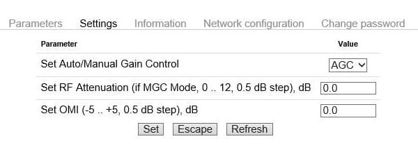
3. Input Sensitivity: The 0.5 Slope Mapping
A critical takeaway from calibration data is the relationship between the RF input drive at the back of the chassis and the resulting modulation depth. There is a precise 0.5 slope between these variables:
ΔIndex (dB) = 0.5 × ΔRF_Input (dB)
Field Breakdown: To increase the OMI by 1dB, the RF input must be raised by 2dB. This 2-for-1 relationship requires precision attenuators. A 1dB error at the input results in a 0.5dB error in the index, which translates back to a 1dB error in the final CNR at the ONU. In high-density subscriber pools, this 1dB difference often defines the margin between a stable link and intermittent “macro-blocking” during peak hours.
4. Field Calculation: Determining Index from DC Current
Without a specialized meter, engineers calculate the index by measuring the DC photocurrent and RF power at the optical receiver. This is the most accurate field verification method.
m = √ [
2 × Prf_wattsRload × (Idc × Responsivity)2
]
Where Prf_watts is the single-channel power, Rload is 75 Ohms, and Responsivity is photodiode efficiency (typically 0.85 to 0.9 A/W). Understanding this formula allows technicians to “see” the laser’s performance through the receiver’s metrics, bypasses guesswork, and identifies whether a failure is due to a weak source or a noisy amplifier chain.
5. Strategic Engineering: The Nonlinearity Threshold
The OMI management is essentially a hunt for the “Sweet Spot.” When we analyze high-power 1550nm EDFAs cascaded with EYDFAs, the noise floor becomes complex. Pushing the index too hard doesn’t just cause clipping; it accelerates Laser Chirp in direct modulation systems. This chirp, interacting with fiber dispersion, creates phase noise that destroys the constellation map (MER) even if the CNR looks perfect.
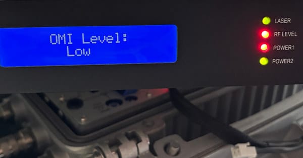
In humid or high-temperature environments (common in South/Southeast Asia), the laser’s threshold current (Ith) may drift. If your OMI is set at the absolute edge of the clipping floor, a 5°C rise in cabinet temperature can push the laser into a non-linear state. We recommend maintaining a “headroom” of at least 1.5dB from the clipping threshold to account for environmental aging and power supply ripple.
6. Detailed Technical Standards Table
| Parameter | Technical Impact of Higher Index | Critical Engineering Limit |
|---|---|---|
| CNR | Improves by 2dB for every 1dB OMI increase. | Receiver Noise Floor. |
| CSO (Second Order) | Degrades rapidly as the laser enters non-linear swing. | Laser P-I Curve Symmetry. |
| CTB (Triple Beat) | Degrades due to third-order non-linearities. | Laser Linearity & Bias Point. |
| Laser Clipping | Occurs when μ (Total Index) > Clipping Threshold. | Threshold Current (I-th). |
| Input RF Sensitivity | 2dB RF change = 1dB OMI change. | AGC Dynamic Range. |
Frequently Asked Questions (Technical FAQ)
Q1: Why does a 1dB change in OMI result in a 2dB change in CNR?
A: Because the modulation index is a voltage-like parameter. At the photodiode, the signal is converted back to the electrical domain where power is proportional to the square of the current (P = I2R). Thus, doubling the index quadruples the RF power.
Q2: What is the recommended Total OMI (μ) to avoid clipping?
A: Most HFC engineers aim for a Total OMI (μ) between 17% and 25%. For digital QAM signals, the threshold is more forgiving, but for legacy analog channels, 21% is the “hard ceiling” to maintain CTB/CSO stability.
Q3: Does OMI change over fiber distance?
A: No. It is an intrinsic property established at the transmitter. While the link’s CNR will drop due to attenuation and fiber noise, the modulation depth remains constant until it is recovered by the receiver’s photodiode.
Conclusion: Precision Calibration for Global Networks
Understanding the Optical Modulation Index is the difference between a carrier-grade network and one plagued by intermittent outages. By respecting the 0.5 slope relationship between RF input and OMI, and the 1:2 ratio for CNR, engineers can deploy Forward Path Transmitters with absolute confidence. Precision in calibration isn’t an option; it’s the foundation of reliability.