


Contents
- The Capacity Problem and the 256QAM Answer
- What 256QAM Demands from Your Network
- Where Does CNR Actually Get Lost?
- Modulation Depth: The One Knob That Moves Everything
- EDFA Noise: Coverage Gain, CNR Pain
- Coax Amplifier Cascades: The Silent Killer
- Putting It Together: System CNR Budget
- What to Adjust First: A Prioritized Checklist
- Frequently Asked Questions
The Capacity Problem and the 256QAM Answer
Cable operators everywhere face the same squeeze. More subscribers want more bandwidth. The spectrum you have is fixed. Building new plant takes years and costs a fortune. So when a change in modulation format promises a 33% capacity increase on the exact same infrastructure, it gets attention.
Here is the math. In the 87–862MHz downstream band, you have 96 channels at 8MHz each. Running 64QAM across all of them gives you roughly 4Gbps of total throughput. Flip to 256QAM and the same channels deliver about 5.34Gbps. That is a 33% bump.
No new fiber. No spectrum reallocation. No truck roll to swap customer equipment. On paper, it looks like the easiest capacity upgrade you will ever do.
Key point: 256QAM gives you 33% more throughput in the same 87–862MHz spectrum. But it demands a higher carrier-to-noise ratio at every point in the signal chain. If your CNR is marginal at 64QAM, it will fail at 256QAM.
And that is the catch. 256QAM is not free. It needs cleaner signals, quieter amplifiers, and more careful power budgeting at every stage. Flip the modulation switch without doing the engineering work, and your error rates will spike. Customers will notice.
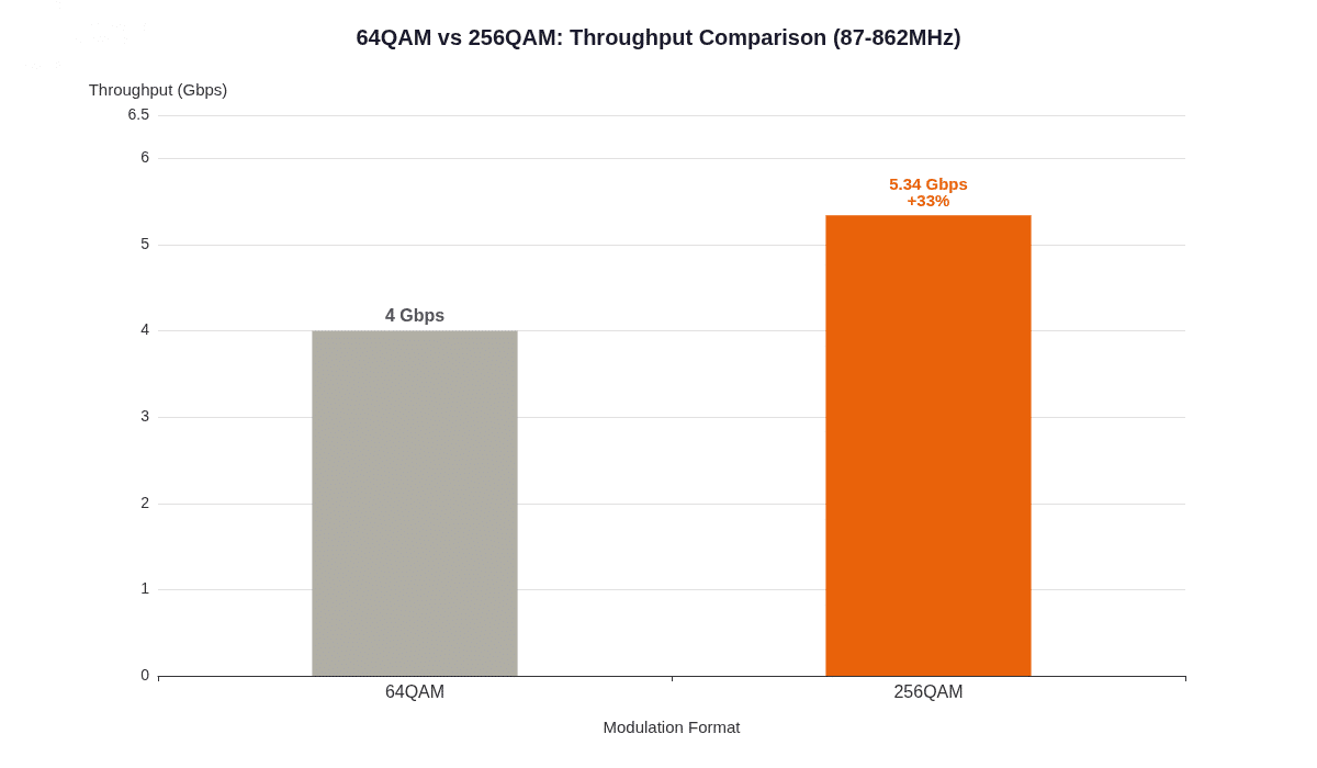
Figure 1: 64QAM vs 256QAM Capacity Comparison
At premlink, we see operators run into this over and over. They change the modulation order, errors climb, and then they spend weeks tracking down the root cause. That root cause is almost always insufficient CNR margin somewhere in the chain. This guide lays out the full picture so you can plan the move to 256QAM with eyes open.
What 256QAM Demands from Your Network
Before you touch any equipment, know the target. IEC 60728-1 defines the electrical performance your system output must meet for 256QAM. These are not suggestions. They are the line between reliable reception and customer complaints.
| Parameter | IEC 60728-1 Requirement | What It Means in Practice |
|---|---|---|
| Maximum output level | 74 dBμV | Do not exceed this at the subscriber tap |
| Minimum output level | 54 dBμV | Signal must stay above this floor |
| Minimum C/N ratio | 32 dB | This is the critical threshold for 256QAM |
| Maximum BER | 2 × 10⁻⁴ | Pre-FEC error rate limit |
| Maximum tilt | 12 dB | Level variation across the full band |
| Adjacent channel level difference | 3 dB | Keep neighboring channels close in level |
| Analog-digital level difference | 6 dB | Digital carriers run below analog |
Most of these numbers fit within what well-maintained HFC plants already deliver. The one that bites you is CNR. Going from 64QAM to 256QAM raises the minimum C/N requirement to 32dB. If your network sits at 33dB today, you have only 1dB of headroom. Temperature drifts, connectors age, and suddenly you are below the threshold.
CNR also drives BER directly. When CNR drops below spec, bit errors climb fast. Unlike analog TV where a noisy picture is still watchable, digital services either work or they do not. There is no graceful degradation with 256QAM. You meet the CNR target, or your customers see artifacts and dropouts.
Where Does CNR Actually Get Lost?
A typical 256QAM HFC network has three physical segments. Signal quality at the subscriber tap is the result of noise accumulated through all three. Understanding which segment contributes the most noise tells you where to focus your optimization effort.
Figure 2: HFC Network Signal Flow and CNR Contribution Chain
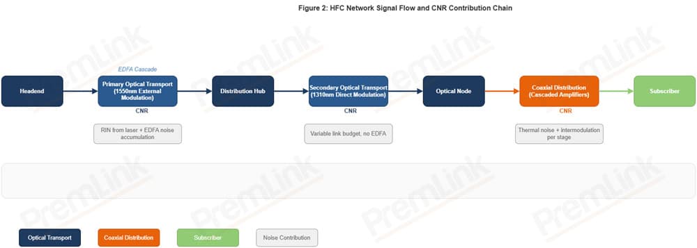
The primary optical link runs from the headend to distribution hubs on 1550nm external modulation. It often includes EDFA amplifiers to cover large areas from a single laser. Each EDFA adds noise. The more stages you cascade, the worse the accumulated relative intensity noise (RIN) gets.
The secondary optical link distributes from hubs to neighborhood optical nodes on 1310nm direct modulation. No EDFA here, but the link budget is less controlled. Fiber runs vary in length. Received optical power can swing several dB between nodes.
The coax distribution runs from the optical node to subscribers through cascaded amplifiers. Each amplifier adds thermal noise and intermodulation products. More stages mean more noise and more tilt across the band.
Here is the thing that surprises people: the noisiest segment dominates your system CNR. If your primary fiber link sits at 48dB CNR but your coax runs at 40dB, the coax sets your performance ceiling. Fixing the fiber will not help much. You have to fix the coax.
System CNR aggregates like this:
Formula (9): System CNR Aggregation
CNR₁ = input signal, CNR₂ = primary fiber, CNR₃ = secondary fiber, CNR₄ = cable network. The 10dB subtraction on CNR₃ accounts for digital carrier modulation depth being lower than analog.
That 10dB penalty on the secondary fiber term is not arbitrary. Digital carriers run at lower RF level than analog carriers. This reduces their modulation depth, which reduces their carrier power relative to noise. The formula captures that reality.
Modulation Depth: The One Knob That Moves Everything
Optical modulation depth is the single most important parameter you can adjust. It determines how much signal power you push onto the fiber, and that directly sets your CNR. Too little depth, and you waste carrier power. Too much, and you clip the laser, causing distortion that no amount of downstream filtering can fix.
The relationship starts simple. If all carriers have the same modulation depth, total modulation depth M relates to per-carrier depth mk and carrier count k like this:
Formula (2): Total Modulation Depth vs Per-Carrier Depth
M = total modulation depth, k = number of carriers, mk = per-carrier modulation depth.
Real networks run mixed analog and digital carriers, so the formula expands:
Formula (3): Mixed Analog-Digital Modulation Depth
ka = analog carrier count, ma = analog modulation depth, kd = digital carrier count, md = digital modulation depth.
Digital carriers run at lower RF level than analog. The standard practice is 10dB below analog. That level difference changes the modulation depth relationship:
Formula (4): Modulation Depth vs RF Level Difference
X = analog-digital RF level difference in dB. With X = 10dB, md ≈ 0.316 × ma.
When X = 10dB, you can simplify the mixed formula into something easier for field use:
Formula (5): Simplified Mixed Transmission (X = 10dB)
Plug in your carrier counts and target total modulation depth, and solve for ma directly.
What the Numbers Look Like in Practice
Take a typical channel plan: 93 channels in the 87–862MHz band, with 8 analog and 85 digital carriers. Here are the calculated values from industry laboratory reference data:
For 1550nm external modulation (M = 0.28):
- Analog modulation depth: 6.9%
- Digital modulation depth: 2.2%
- Analog RF level: 87.07 dBμV per channel
- Digital RF level: 77.07 dBμV per channel (10dB below analog)
For 1310nm direct modulation (M = 0.30):
- Analog modulation depth: 7.4%
- Digital modulation depth: 2.36%
- Reference RF level: 75 dBμV per channel (84 PAL D/K basis)
- Analog RF level: 82.07 dBμV per channel
- Digital RF level: 72.07 dBμV per channel
Notice the 1310nm link runs a slightly higher total modulation depth (0.30 vs 0.28). This compensates for the noise added in downstream distribution amplifiers. But it also means the 1310nm laser is closer to its clipping limit. You need to be careful not to overdrive it.
When Your Channel Count Changes
Networks do not stay static. You add or remove channels over time. When that happens, RF drive levels must change to keep total modulation depth constant. The adjustment formula is straightforward:
Formula (6): RF Level Adjustment for Channel Changes
K = number of loaded channels. Fewer channels → raise per-channel level. More channels → lower it.
If you remove channels and do not raise the remaining drive levels, you leave CNR on the table. If you add channels without reducing per-channel power, you risk clipping. Neither is good for 256QAM.
EDFA Noise: Coverage Gain, CNR Pain
EDFAs make economic sense for HFC. One optical amplifier can replace dozens of coax distribution amplifiers. Fewer active devices mean lower maintenance costs and better reliability. But EDFAs add noise, and that noise accumulates with each stage.
The core issue is relative intensity noise. Each EDFA stage adds RIN. The next stage amplifies that RIN along with the signal. The accumulated output RIN of a multi-stage EDFA cascade follows this relationship:
Formula (7): Cascaded EDFA Output RIN
E = 1.278 × 10⁻¹⁶ mJ (photon energy at 1550nm), NFk = noise figure of stage k, Pkin = input power of stage k, RINkin = input RIN of stage k.
This formula tells you something important: noise accumulation depends on each stage’s noise figure and input power. If a later stage receives degraded input power, it adds disproportionately more noise than the formula suggests on paper.
A Real Example
Consider a two-stage EDFA setup from industry laboratory measurements. The first stage output (point B) delivers 4.8dBmW. The second stage output (point C) delivers 5dBmW. Both stages have noise figures around 6.5dB. Running through the formula gives RINout ≈ -149.77 dB(Hz)⁻¹.
Without EDFA, the same 1550nm link would show RIN around -155 dB/Hz. That is a 5+ dB noise penalty just from adding two EDFA stages. In a 256QAM system where you are fighting for every decibel of CNR, that is a big deal.
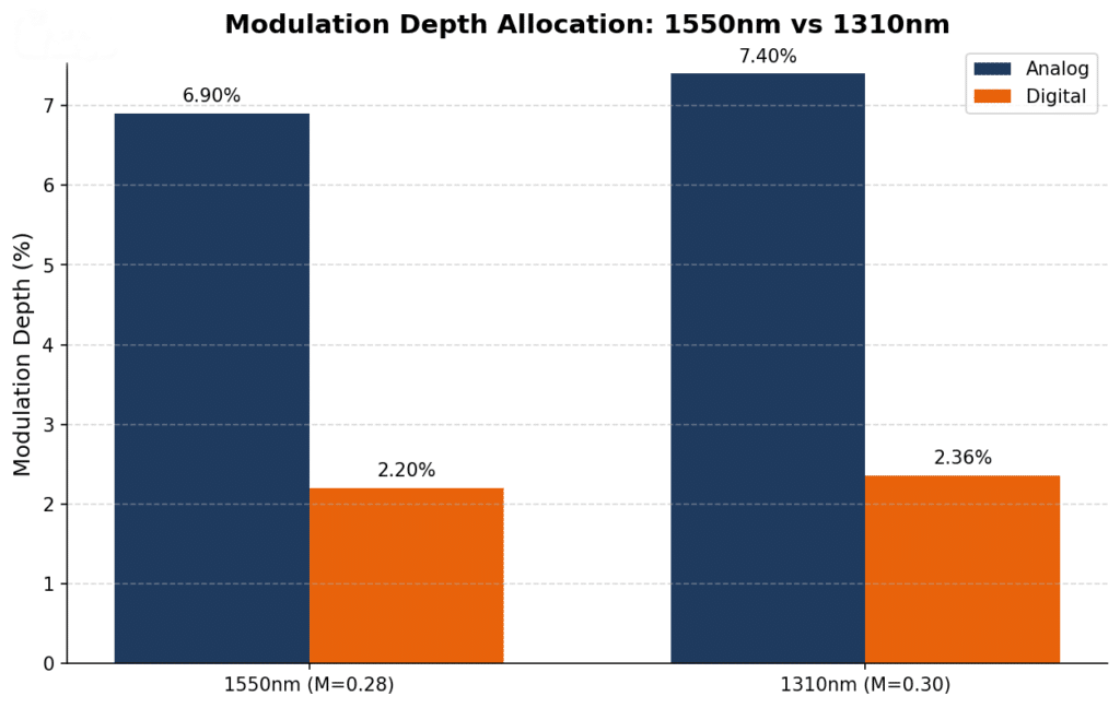
Figure 3: 1550nm CNR vs RF Drive Level (No EDFA)
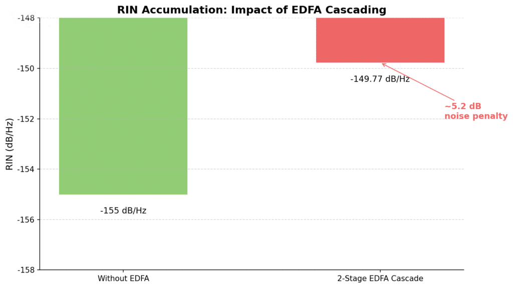
Figure 4: 1550nm CNR vs Received Optical Power (With EDFA)
Design rule: When received optical power goes above -7dBmW, EDFA noise starts dominating your noise budget. Keep EDFA input power in the 0 to -7dBmW sweet spot for 256QAM. Also, industry laboratory testing shows that 1550nm reference drive points typically sit 1dB below the CNR peak. You have room to push RF drive levels higher before clipping.
EDFA Guidelines for 256QAM
- Minimize cascade stages. Each EDFA adds noise. If you need more than two stages, rethink your fiber routing.
- Keep input power above -7dBmW. Below this, noise contributions accelerate quickly.
- Measure RIN at commissioning. Baseline measurements let you track degradation over time. RIN drift signals aging components or power instability.
- Leave 3dB of link margin. Temperature swings and connector aging will eat your margin. Plan for it.
Coax Amplifier Cascades: The Silent Killer
The coax distribution network gets less attention than fiber, but it often determines whether 256QAM works or fails. Each amplifier in a cascade adds thermal noise and intermodulation products. More stages compound both problems in ways that devastate high-order modulation.
Let us be blunt: for 256QAM, keep your amplifier cascades to four stages or fewer. This is not a guideline you can bend. Four stages match the performance of fiber-deep architectures across the full 87–862MHz band. Five stages degrade frequencies above 650MHz by 1–2dB. Six or more stages push performance into unacceptable territory.
Field reality: If your plant runs more than four amplifier stages between the optical node and the subscriber, 256QAM will not work reliably. No amount of level tweaking fixes excessive cascade depth. You need node segmentation or fiber extension.
Amplifier Noise Math
IEC specifies minimum 45dB CNR for cable networks in MDU (multi-dwelling unit) environments. The cable network CNR follows:
Formula (8): Cable Network CNR
Si = cable network input level (75 dBμV), F = amplifier noise figure (10 dB), n = number of cascade stages.
With Si = 75 dBμV and F = 10 dB, you can calculate CNR for different cascade depths:
| Cascade Stages | CNR (dB) | Meets 45dB MDU Spec? |
|---|---|---|
| 2 | 57.6 | Yes, with large margin |
| 4 | 51.6 | Yes |
| 6 | 48.6 | Yes, but tight |
| 10 | 44.6 | No — below 45dB spec |
Those numbers look like you could run 6 or even 8 stages and still hit 45dB. But CNR is only half the story. Distortion products also accumulate with cascade depth, and they hit 256QAM carriers harder than the CNR math suggests.
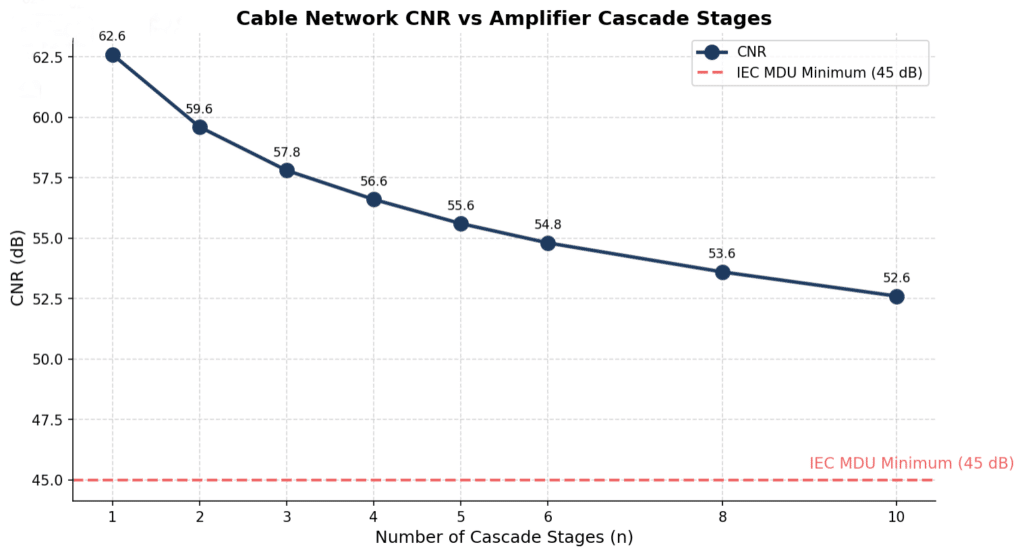
Figure 5: Frequency Response vs Amplifier Cascade Depth
Industry laboratory measurements confirm this. Four amplifier stages keep the frequency response flat across 87–862MHz. Five stages introduce 1–2dB droop above 650MHz. Six or more stages show divergent roll-off that makes 256QAM on upper channels impossible. Cable attenuation increases with frequency, and each amplifier stage adds tilt compensation error that accumulates. Passive splitters and taps make it worse because their high-frequency loss exceeds theoretical predictions.
Putting It Together: System CNR Budget
Individual segment performance does not guarantee end-to-end performance. You have to budget CNR across all segments. This is where many 256QAM deployments stumble. Engineers optimize each segment in isolation and miss the aggregate.
The IEC CNR formula for individual optical links is the foundation:
Formula (1): IEC Optical Link CNR
BN = noise bandwidth, mk = per-carrier modulation depth, R = receiver responsivity, Pr = received optical power, RIN = relative intensity noise, e = electron charge, Id0 = dark current, Ieq = equivalent input noise current.
This formula separates signal power from three noise sources: laser RIN, shot noise (from dark current and photocurrent), and receiver thermal noise. Signal power depends on modulation depth and received optical power. If either drops, CNR drops with it.
A Worked Example
Let us plug in realistic values and see what the system CNR looks like:
- Input signal CNR for analog: 50 dB
- Input signal CNR for 256QAM: 37.9 dB
- Primary fiber CNR (two-stage EDFA, 0dBmW received): ~50 dB
- Secondary fiber CNR (1310nm, -5dBmW received): ~48 dB
- Cable network CNR (4-stage cascade): ~52 dB
- Analog-digital level difference: 10 dB
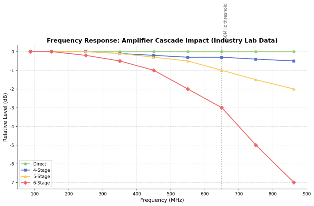
Figure 6: System Output CNR vs Secondary Fiber Received Power
Running through the system CNR aggregation formula, the result lands around 35–37dB for the digital carriers. That gives you 3–5dB of margin above the 32dB IEC minimum. Not luxurious, but workable. If any segment degrades by even 2–3dB, you lose your margin.
The key insight from this exercise: secondary fiber received optical power is the binding constraint. When it drops below -10dBmW, system CNR for 256QAM falls below the 32dB threshold. This is where you need the most careful engineering.
What to Adjust First: A Prioritized Checklist
Here is what to actually do, in order of impact and effort.
Priority 1: Primary Fiber RF Drive Levels
Your headend settings affect everything downstream. Get these right first:
- Push RF drive toward full modulation. Industry laboratory testing shows that typical 1550nm platforms run about 1dB below the CNR peak at reference settings. You have room to increase drive levels. Use it.
- Control EDFA input power to 0–3dBmW. Below -7dBmW, EDFA noise starts eating your CNR budget.
- Track RIN over time. Baseline at commissioning. RIN drift predicts failures before they affect customers.
Priority 2: Secondary Fiber Settings
This segment often gets less attention. That is a mistake:
- Do not run at the clipping limit. The 1310nm link is closer to its modulation ceiling than the 1550nm link. Leave 2–3dB of headroom to prevent digital peak clipping.
- Keep received optical power above -10dBmW. This is the hard floor. Below it, your system CNR budget fails.
- Account for variable fiber lengths. Secondary links serve different distances. Budget optical power for the longest run, not the average.
Priority 3: Coax Cascade Reduction
If your cascade exceeds four stages, no adjustment helps. You need physical changes:
- Count your amplifier stages. If you find five or more between node and subscriber, plan a segmentation project.
- Extend fiber deeper. Moving the optical node closer to subscribers eliminates cascade stages without adding cabinet equipment.
- Upgrade old amplifiers. Modern push-pull and GaAs amplifiers offer better noise figures and lower distortion than legacy modules.
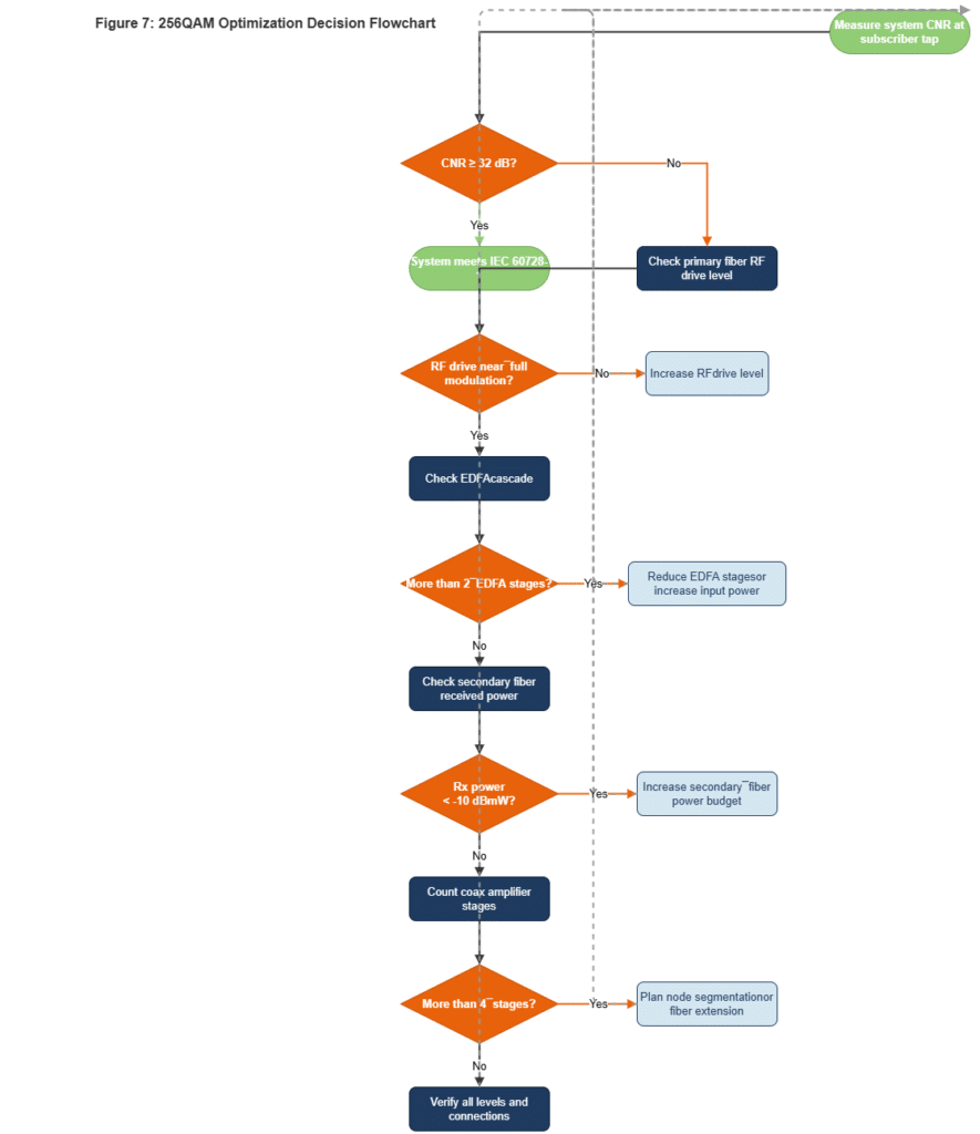
Figure 7: 256QAM Optimization Decision Flow
Priority 4: Ongoing Monitoring
Optimization is not a one-and-done activity:
- Set baselines. Measure CNR, MER, and BER at key nodes when everything is working right.
- Watch trends, not just thresholds. A 1dB CNR decline over six months predicts problems. Fix it before customers notice.
- Adjust for seasons. Laser output and fiber loss change with temperature. In extreme climates, seasonal level adjustments may be necessary.
As we emphasize at premlink.net, the difference between networks that successfully deploy 256QAM and those that struggle comes down to margin management. The 33% capacity gain is real, but it lives inside a narrow CNR window. Protect that window, and the upgrade pays for itself. Ignore it, and you spend more on troubleshooting than you saved on the modulation change.
Frequently Asked Questions
Q:How much capacity does 256QAM add over 64QAM in HFC networks?
A: In the 87–862MHz band with 96 channels of 8MHz each, 64QAM gives you about 4Gbps. 256QAM pushes that to roughly 5.34Gbps. That is a 33% gain on the same spectrum, the same fiber, the same coax.
Q: What minimum CNR does IEC 60728-1 require for 256QAM?
A: IEC 60728-1 sets the minimum carrier-to-noise ratio at 32dB for 256QAM at the system output. Other requirements include maximum output level 74dBμV, minimum output level 54dBμV, maximum tilt 12dB, adjacent channel level difference 3dB, and analog-digital level difference 6dB.
Q: Why does EDFA make CNR worse in 1550nm HFC links?
A: Each EDFA stage adds relative intensity noise (RIN). A two-stage EDFA cascade raises RIN from about -155dB/Hz to roughly -149.77dB/Hz. That 5+ dB noise penalty eats into your CNR budget. When received optical power goes above -7dBmW, EDFA noise starts dominating the total noise floor.
Q: How many coax amplifier stages can a 256QAM HFC network tolerate?
A: Keep it to four stages or fewer. Four stages match fiber-deep performance across 87–862MHz. Five stages degrade frequencies above 650MHz by 1–2dB. Six or more stages make 256QAM unreliable.
Q: What is the system-level CNR formula for HFC networks?
A:
where CNR1 through CNR4 are input signal, primary fiber, secondary fiber, and cable network CNR values. The 10dB subtraction on CNR3 accounts for the digital carrier modulation depth penalty.
Q: What optical receive power should I target for 256QAM?
A: For 1550nm links with EDFA, aim for 0 to +3dBmW. For 1310nm secondary links, stay above -10dBmW. Always leave headroom—running at the minimum leaves no room for aging, temperature swings, or fiber connector degradation.
Q: How does analog-digital level difference affect modulation depth?
A: Digital carriers run 10dB below analog carriers. The modulation depth relationship is
With X=10dB, digital modulation depth is about 31.6% of analog depth. IEC 60728-1 specifies a 6dB analog-digital level difference for 256QAM systems.
Q: Can I run 256QAM across the full 87-862MHz band on existing HFC plant?
A: Yes, but only if your CNR budget clears 32dB at every system output point. That means optimizing RF drive levels, managing EDFA cascade noise, keeping amplifier stages to four or fewer, and maintaining proper optical power budgets. It is not a software switch—it requires engineering work.
About premlink.net: This guide is part of premlink.net’s technical library for the CATV optical communications industry. Find more products, such as optical transmitter, EDFA at our products center.