The post Premlink is Heading to Jakarta for INTI 2026! appeared first on Premlink - Homepage.
]]>The countdown is on! We are excited to announce that Premlink Tech is heading to Jakarta to participate in INTI 2026 (Indonesia Technology & Innovation)—the region’s landmark event for the emerging intelligent era.
If you are attending, we’d love for you to drop by, grab a coffee, and talk optical tech with us.
- Where to find us: Booth A3-34A
- Venue: Jakarta International Expo (JIExpo), Indonesia
- When: August 11–13, 2026
What We Are Bringing to Jakarta INTI
We know that building stable optical networks in Southeast Asia comes with unique challenges—especially dealing with high humidity, high temperatures, and the constant demand for cost-effective bandwidth upgrades.
At our booth, we’ll be showcasing some of our most practical, field-tested hardware designed to solve these exact issues:
- Multi-Port High-Power EDFAs: Optimized for GPON/XGSPON/50GPON co-existence, helping ISPs deliver high-quality RF overlay without losing signal integrity.
- Reliable WDM CATV Optical Receivers : Optimized for GPON/XGSPON/50GPON co-existence as well.
Let’s Connect!
We believe in practical engineering and reliable manufacturing. Whether you are a local ISP, a telecom distributor, or a CATV system integrator, we want to hear about your current network challenges and see how our agile OEM/ODM solutions can help.
Stop by Booth A3-34A to check out our live hardware demos and chat directly with our team.
If you’d like to book a specific time slot to sit down and discuss a project, feel free to drop us a quick line at sales#premlink.net.
See you in Jakarta!

Learn more about our product lineup at: www.premlink.net
The post Premlink is Heading to Jakarta for INTI 2026! appeared first on Premlink - Homepage.
]]>The post PL150D-5 in GPON + XGS-PON Coexistence Architecture: Migration Guide for FTTH Operators appeared first on Premlink - Homepage.
]]>In this guide
- Why GPON and XGS-PON need to coexist, not replace each other
- The wavelength plan: who gets what
- What the PL150D-5 actually does in coexistence mode
- Optical isolation budget for the coexistence case
- Three realistic migration paths
- RFoG + XGS-PON coexistence
- Looking ahead: 25G / 50G PON joining the same fiber
- When the PL150D-5 is not enough
- Frequently asked questions
Why GPON and XGS-PON need to coexist, not replace each other
Most FTTH operators built out their networks on GPON between 2010 and 2018. By 2026, a meaningful share of those subscribers are on 1 Gbps plans and the GPON upstream (1.25 Gbps shared) and downstream (2.5 Gbps shared) are filling up. The upgrade path most operators choose is XGS-PON, which delivers 10 Gbps symmetric per wavelength.
A forklift replacement is not realistic. Splitter cabinets, drop fibers, and inside wiring are already in place. Most operators want a coexistence model where GPON subscribers keep their ONUs until they are individually upgraded, while XGS-PON subscribers on the same ODN use a different wavelength pair. The two services share the same physical fiber, the same splitter, and the same home-side WDM receiver in the FTTH triple-play case.
The PL150D-5 FTTH XGSPON optical receiver is built around a wide-band thin-film filter that reflects 1550 nm toward the receiver photodiode and passes everything from 1260 to 1500 nm and 1575 to 1580 nm to the ONU port. That wide pass band is what makes the device compatible with both GPON and XGS-PON simultaneously. The same filter design also leaves room for 25G PON (1342 nm upstream) and 50G PON in the same channel. The headend side of the same architecture is covered in the XGS-PON EDFA pass-through guide.
The wavelength plan: who gets what
| Service | Downstream (nm) | Upstream (nm) | Standard |
|---|---|---|---|
| CATV broadcast | 1540–1560 | — | — |
| GPON | 1480–1500 | 1260–1360 (centered on 1310) | ITU-T G.984 |
| XGS-PON | 1575–1580 | 1260–1280 (centered on 1270) | ITU-T G.9807.1 |
| 25G PON | 1340–1344 (downstream option) | 1290–1310 (centered on 1300) | ITU-T G.9804 |
| 50G PON (planned) | 1342–1344 | 1300–1320 | ITU-T G.9804 (draft) |
Three observations matter for the receiver design.
First, GPON upstream (centered 1310 nm) and XGS-PON upstream (centered 1270 nm) are 40 nm apart. A wide enough filter can pass both, which is what the PL150D-5 reflect channel does at 1260–1500 nm.
Second, GPON downstream (1490 nm) and XGS-PON downstream (1577 nm) are 87 nm apart. A single thin-film filter can pass both if the band is wide enough. The PL150D-5 reflect channel includes 1575–1580 nm for this reason.
Third, 25G PON lands in the 1290–1344 nm range, overlapping both GPON upstream (1310 nm) and XGS-PON upstream (1270 nm) at the edges. The PL150D-5 reflect band (1260–1500 nm) covers 25G PON as well, but a 25G PON ODN must use a narrower wavelength plan to avoid interfering with live GPON.
What the PL150D-5 XGSPON Optical Receiver actually does in coexistence mode

In a coexistence install the device sits between the drop fiber and the ONU, handling three wavelengths at once.
| Wavelength (nm) | Service | What the receiver does |
|---|---|---|
| 1270 | XGS-PON upstream | Passes through to ONU port (≤ 1.0 dB IL, ≥ 35 dB isolation from 1550 nm) |
| 1310 | GPON upstream | Passes through to ONU port (≤ 1.0 dB IL, ≥ 35 dB isolation from 1550 nm) |
| 1490 | GPON downstream | Passes through to ONU port (≤ 1.0 dB IL) |
| 1550 | CATV broadcast | Reflects to photodiode, converts to RF (47–1002 MHz) |
| 1577 | XGS-PON downstream | Passes through to ONU port (≤ 1.0 dB IL) |
The relevant numbers are documented in the PL150D-5 XGSPON optical receiver datasheet: ≤ 1.0 dB insertion loss on both pass and reflect channels, ≥ 35 dB optical isolation at 1310 nm, ≥ 30 dB isolation at 1490 / 1577 nm, ≥ 18 dB isolation at 1550 nm. In a coexistence ODN, the 1310 nm isolation is the most important number, because the GPON upstream burst and the 1550 nm broadcast carrier share the same pass port and cannot leak into each other.
For the AGC window (−10 to 0 dBm) and the optical input range (−15 to +2 dBm), the device behaves identically to a single-PON install. The coexistence case does not change the in-home optical power budget for the 1550 nm carrier. The 1270, 1310, 1490, and 1577 nm carriers all pass through with the same loss regardless of which PON service the subscriber is on. The headend platform is on the Premlink WDM PON EDFA/EYDFA page.
Optical isolation budget for the coexistence case
In a coexistence ODN, the four upstream/downstream wavelengths that share the PL150D-5 COM port have to be separated cleanly:
At COM port:
  1310 nm burst (GPON upstream)         → pass to ONU port    : ≥ 35 dB isolation from 1550 nm
  1270 nm burst (XGS-PON upstream)      → pass to ONU port    : ≥ 30 dB isolation from 1577 nm
  1490 nm carrier (GPON downstream)      → pass to ONU port    : ≤ 1.0 dB IL
  1577 nm carrier (XGS-PON downstream)  → pass to ONU port    : ≤ 1.0 dB IL
  1550 nm carrier (CATV)                → reflect to detector : ≤ 1.0 dB IL, AGC −10 to 0 dBm
The two figures that matter for coexistence are the 1310 nm isolation (≥ 35 dB) and the 1550 nm isolation (≥ 18 dB). The 1310 nm number protects the GPON upstream laser from 1550 nm leakage; the 1550 nm number protects the receiver photodiode from back-reflected 1550 nm signal that would otherwise raise the receiver noise floor and degrade CTB / CSO / C/N. Both figures are on the PL150D-5 datasheet.
The coexistence case also adds a third consideration: the WDM shelf at the headend has to combine and split the 1490 / 1577 / 1550 nm downstream wavelengths, and it has to pass the 1270 / 1310 nm upstream bursts in the opposite direction. The XGS-PON EDFA platform and the WDM PON EDFA/EYDFA family are designed for that filter stack. The receiver’s compatibility with both GPON and XGS-PON only matters if the headend can deliver both wavelengths to the same ODN.
Three realistic migration paths
Path 1 — Overlay, same ODN. Add an XGS-PON OLT to the existing GPON OLT, with a WDM shelf that combines 1490 and 1577 nm onto the same fiber. Existing GPON subscribers stay on their current ONUs. New XGS-PON subscribers are provisioned on a new wavelength pair. The PL150D-5 receiver handles either service without change. This is the lowest-cost migration path and the most common in 2026 deployments.
Path 2 — Move GPON to 1577 nm (XGS-PON band). A small number of operators are migrating GPON traffic to the XGS-PON wavelength pair, freeing the 1490 nm band for future use. This requires changing every subscriber’s ONU but does not change the drop fiber or the home-side WDM receiver. The PL150D-5 reflect band covers both 1490 and 1577 nm with the same insertion loss, so the receiver does not need to be replaced.
Path 3 — Coexistence with 25G PON. The 25G PON wavelength plan lands upstream in 1290–1310 nm, which overlaps GPON upstream (1310 nm) at the band edge. Most operators rolling out 25G PON will do so on a new ODN or by re-using the 1577 nm downstream band with a different upstream wavelength. The PL150D-5 reflect band (1260–1500 nm) covers the 25G PON upstream range, but operators should confirm with the vendor that the reflect band flatness holds across 1260–1344 nm before specifying in a 25G PON deployment.
RFoG + XGS-PON coexistence
RFoG (Radio Frequency over Glass) is a 1550 nm downstream + 1610 nm upstream architecture used by some North American MSOs. It shares the same 1550 nm broadcast spectrum as FTTH triple-play, but the upstream is on a different wavelength (1610 nm instead of 1270/1310 nm).
The PL150D-5 xgspon optical receiver reflect channel is 1260–1500 nm and 1575–1580 nm, which does not cover 1610 nm. For pure RFoG deployments, a different receiver with a wider reflect band is required. For mixed RFoG + XGS-PON deployments where some subscribers are on RFoG and others on XGS-PON, the same ODN requires a different filter stack at the headend and a different receiver at the RFoG subscribers’ premises. The PL150D-5 is the right choice for the XGS-PON side of the mixed deployment.
Looking ahead: 25G / 50G PON joining the same fiber
25G PON and 50G PON are landing in the 1290–1344 nm upstream range, with 25G PON currently specified at 1300 nm center and 50G PON in the 1342–1344 nm range. Both overlap the existing GPON upstream (1310 nm) and XGS-PON upstream (1270 nm) at the band edges. The PL150D-5 xgspon optical receiver reflect band (1260–1500 nm) covers the 25G and 50G PON upstream lanes, but the wider ODN must use a wavelength plan that prevents collisions with live GPON and XGS-PON services. The WDM PON EDFA/EYDFA family covers the headend side.
In practice, the most likely 2026–2028 deployment pattern is:
- Keep GPON on 1310 nm upstream / 1490 nm downstream
- Add XGS-PON on 1270 nm upstream / 1577 nm downstream
- Add 25G PON on a new 1342 nm upstream lane, with the 1577 nm downstream shared with XGS-PON or moved to a new band
The PL150D-5 xgspon optical receiver reflect band covers all three services in the upstream direction. The downstream coexistence gets harder as more services share the 1575–1580 nm range, so operators will need to plan the headend WDM filter stack carefully.
When the PL150D-5 XGSPON optical receiver is not enough
Three coexistence scenarios are out of scope for the PL150D-5 xgspon optical receiver.
1. RFoG upstream at 1610 nm. The PL150D-5 xgspon optical receiver reflect channel stops at 1500 nm. RFoG subscribers need a receiver with a 1610 nm pass port.
2. RF output above 1002 MHz. The PL150D-5 xgspon optical receiver RF frequency range is 47–1002 MHz. DOCSIS 4.0 R-PHY architectures that push 1.2 GHz or 1.8 GHz need a wider receiver or a downstream in-home RF amplifier. The headend side is covered in the EDFA noise-figure guide.
3. Outdoor plant with wide temperature spec. The PL150D-5 xgspon optical receiver operating temperature is −10 to +50 °C. Outdoor enclosures in cold climates may need an extended-temperature variant. Confirm with the vendor before specifying for outdoor use.
For everything else, the PL150D-5 xgspon optical receiver is the home-side anchor of the FTTH triple-play coexistence architecture. The full specifications are on the PL150D-5 xgspon optical receiver page. Lead time is 15 days for 100 pcs / 25 days for 5,000 pcs / negotiable above 5,000 pcs.
Frequently asked questions
Q1. Can GPON and XGS-PON share the same fiber?
Yes. ITU-T G.984 (GPON) and ITU-T G.9807.1 (XGS-PON) are designed to coexist on the same ODN. GPON uses 1310 nm upstream and 1490 nm downstream; XGS-PON uses 1270 nm upstream and 1577 nm downstream. The wavelengths do not collide, and a WDM shelf at the headend combines them onto the same fiber. The PL150D-5 is documented on the Premlink FTTH WDM receiver product page.
Q2. Does the home-side WDM receiver need to change when XGS-PON is added?
No. The PL150D-5 xgspon optical receiver reflect channel covers 1260–1500 nm and 1575–1580 nm, which includes both GPON (1310 / 1490 nm) and XGS-PON (1270 / 1577 nm). The pass-channel insertion loss is ≤ 1.0 dB for both services, so the ONU upstream budget is not degraded by sharing the receiver. The same receiver works for GPON-only, XGS-PON-only, and coexistence subscribers.
Q3. What is the optical isolation between GPON upstream and the 1550 nm CATV carrier?
The PL150D-5 xgspon optical receiver pass-port isolation at 1550 nm is ≥ 18 dB, which means the 1550 nm broadcast carrier does not leak into the GPON upstream path. The reflect-port isolation at 1310 nm is ≥ 35 dB, so the GPON upstream burst is not contaminated by 1550 nm back-reflection. The full spec is on the PL150D-5 datasheet.
Q4. Can I run XGS-PON and 25G PON on the same fiber at the same time?
The 25G PON upstream wavelength (1290–1310 nm) overlaps GPON upstream (1310 nm) at the band edge. A combined XGS-PON + 25G PON ODN requires careful wavelength planning and a WDM filter stack at the headend that separates the two upstream lanes. The PL150D-5 reflect band covers the 25G PON upstream range, but operators should confirm flatness with the vendor before specifying in a 25G PON deployment.
Q5. What is the migration cost to add XGS-PON to an existing GPON ODN?
The minimum cost path is to overlay: add an XGS-PON OLT, add a WDM shelf that combines 1490 and 1577 nm downstream and separates 1270 and 1310 nm upstream, and provision new XGS-PON subscribers on the new wavelength pair. Existing GPON subscribers keep their current ONUs. The drop fiber, splitter, and home-side WDM receiver (PL150D-5) do not change. The headend platform is on the XGS-PON EDFA product page.
Q6. Can the PL150D-5 support RFoG and XGS-PON on the same ODN?
The PL150D-5 xgspon optical receiver reflect channel is 1260–1500 nm and 1575–1580 nm, which does not include the RFoG upstream wavelength of 1610 nm. For mixed RFoG + XGS-PON ODNs, RFoG subscribers need a different receiver with a 1610 nm pass port, and the headend WDM filter stack has to accommodate both upstream bands. The XGS-PON side of the ODN can use the PL150D-5 unchanged.
Q7. Will the home-side receiver need to be replaced for 25G PON?
For 25G PON upstream (1290–1310 nm), the PL150D-5 xgspon optical receiver reflect band is wide enough. For 50G PON upstream (1342–1344 nm), the reflect band also covers it. The downstream side is more complex, because 25G / 50G PON may share the 1575–1580 nm range with XGS-PON. Confirm the downstream coexistence plan with the headend vendor before specifying.
Q8. What is the lead time and MOQ for the PL150D-5 xgspon optical receiver?
Standard lead time is 15 days for 100 pcs, 25 days for 5,000 pcs, and negotiable for volumes above 5,000 pcs. Sample MOQ is 1 pc. Custom labels and temporary logos are available from 1 pc MOQ. Confirm current lead time with the vendor before placing the order; the product page has the latest figure.
About the author. The Premlink Optical Networking Team designs and specifies FTTH WDM receivers, EDFA, EYDFA, and WDM shelf products for ISP and carrier networks. Premlink’s product portfolio covers the FTTH XGSPON optical receiver (PL150D-5), the XGS-PON EDFA platform, the WDM PON EDFA/EYDFA family, and the CATV EDFA/EYDFA platform.
About Premlink. Premlink supplies optical amplification and wavelength management products for broadband access networks. For product datasheets or design support, visit www.premlink.net.
Last updated: 23 June 2026
Reviewed against: Premlink PL150D-5 datasheet (2026 rev.); ITU-T G.984 (GPON), G.987 (XG-PON), G.9807.1 (XGS-PON), G.9804 (25G/50G PON) wavelength plans; commercial FTTH WDM receiver datasheets at 25 °C reference.
Sources & further reading: PL150D-5 FTTH XGSPON optical receiver product page · PL150D-5 xgspon optical receiver overview · High Power EDFA & EYDFA with XGS-PON Pass-Through · EDFA Noise Figure Explained.
The post PL150D-5 in GPON + XGS-PON Coexistence Architecture: Migration Guide for FTTH Operators appeared first on Premlink - Homepage.
]]>The post EDFA Noise Figure Explained: Why It Matters for CATV and FTTH Amplifiers appeared first on Premlink - Homepage.
]]>Quick answer (for AI Overview and featured snippets): EDFA noise figure is the SNR degradation an amplifier adds, expressed in dB. It comes from amplified spontaneous emission (ASE) generated in the erbium-doped fiber. Industry standards (IEC 61290-1, Telcordia GR-1312-CORE) measure NF at 0 dBm input because that point sits in the linear, unsaturated regime where the spec is reproducible across vendors. Typical values: EDFA 4.0–4.5 dB, EYDFA 4.5–5.5 dB. See Premlink’s CATV EDFA/EYDFA product family for datasheet specs.
In this guide
- What noise figure actually means in an optical amplifier
- Why NF matters in EDFA and EYDFA deployments
- Why the NF spec is measured at 0 dBm input
- EDFA vs. EYDFA: a clear NF trade-off
- Five design factors that move NF
- NF impact in real network scenarios
- How to read an NF datasheet
- Looking ahead: NF in next-generation amplifiers
- Frequently asked questions
What Noise Figure actually means in an optical amplifier
Noise figure is the ratio of input signal-to-noise ratio to output signal-to-noise ratio. In linear units it is simply NF = SNRin / SNRout. In decibels it is NF(dB) = SNRin(dB) − SNRout(dB). It tells you, in a single number, how much cleaner the input was than the output, after the amplifier has done its work.
An ideal amplifier would have NF = 0 dB: it would copy the signal without adding any noise of its own. Real optical amplifiers do not. The erbium-doped fiber (or erbium-ytterbium-doped fiber in EYDFA) emits broadband light on its own, even when no signal is present. That light is called amplified spontaneous emission (ASE). ASE sits across the entire C-band, overlaps the signal wavelength, and beats with the signal at the photodetector, producing electrical noise that the receiver cannot separate from the data.
Two practical consequences follow:
- NF is not gain. A 22 dBm EDFA and a 30 dBm EYDFA can have nearly the same NF if they use the same pump structure. Output power and NF are independently specified.
- NF is not output OSNR. OSNR at the receiver is a function of NF, input power, gain, and optical filtering. NF is the amplifier-side contribution to that OSNR.
Why Noise Figure matters in EDFA and EYDFA deployments
Every optical amplifier in the headend adds ASE. Every ASE contribution reduces the signal quality at the optical receiver. Two metrics track that quality:
- CNR (carrier-to-noise ratio) in analog and QAM video distribution
- OSNR (optical signal-to-noise ratio) in digital data transport
For a single amplifier with gain G, the OSNR at the output is approximately:
OSNR_out ≈ P_in − NF − 10·log10(B_opt) + 58
where B_opt is the optical measurement bandwidth (typically 0.1 nm). At a fixed input power, every 1 dB of NF costs you 1 dB of OSNR at the output. That 1 dB translates directly into ~1 dB of CNR at the optical node — or, in a digital PON, into ~1 dB of receiver sensitivity margin.
Cascaded amplifiers: Friis formula for optics
When the optical path goes through two amplifiers (for example, a headend EDFA plus a mid-span EYDFA in a long-reach build), the NFs combine. In optical form, the cascade is:
NF_total ≈ NF1 + (NF2 − 1) / G1
For two 22 dB-gain amplifiers with NF1 = 4.5 dB and NF2 = 5.5 dB:
- NF1 in linear = 2.82
- NF2 in linear = 3.55
- G1 in linear = 158
- NF_total = 2.82 + (3.55 − 1) / 158 = 2.82 + 0.016 = 2.84 in linear ≈ 4.53 dB
The first amplifier dominates the cascade. Improving NF1 by 0.5 dB is worth more than improving NF2 by 2 dB. For deployment guidance, see the WDM PON EDFA/EYDFA platform.
Why the Noise Figure spec is measured at 0 dBm input
Two standards govern the measurement: IEC 61290-1 for general optical amplifiers and Telcordia GR-1312-CORE for telecom-grade EDFAs. Both specify the input signal at 0 dBm (1 mW) into the amplifier under test. There is a practical reason this number won, not an arbitrary one.
Three reasons 0 dBm is the reference
- Above the measurement floor. Optical spectrum analyzers and noise-figure benches have a residual noise floor of about −65 to −70 dBm at 0.1 nm resolution. Driving the amplifier with 0 dBm keeps the output well above that floor, so the NF calculation is not limited by instrument noise.
- Below gain compression. Below roughly −3 dBm input, an EDFA starts to leave the small-signal regime. Pump power is not fully consumed by the signal, and the inversion profile changes with input power. NF drifts upward as input drops.
- Below saturation. Above roughly +3 dBm input, gain saturation kicks in. The amplifier can no longer hold its small-signal gain, output power clips, and the NF calculation breaks down. 0 dBm is comfortably below that knee.
0 dBm is the “sweet spot” where the NF value is at its minimum and reproducible across units, vendors, and test benches. Vendors publish NF at 0 dBm input for that reason. Real headend input is usually between −10 dBm and −3 dBm, so the datasheet number is a conservative best case.
EDFA vs. EYDFA: a clear Noise Figure trade-off
Both amplifier types are doped-fiber devices, but the doping and pump structure differ. That difference is the reason the NF spec is also different.
| Parameter | EDFA | EYDFA |
|---|---|---|
| Active fiber | Erbium-doped, single-cladding | Erbium-ytterbium co-doped, double-cladding |
| Pump wavelength | 980 nm | 915 / 940 nm (multi-mode) |
| Typical NF @ 0 dBm input | 4.0–4.5 dB | 4.5–5.5 dB |
| Typical small-signal gain | 15–25 dB | 20–30 dB |
| Maximum total output | ~27 dBm | 27–33 dBm |
| Best fit | CNR-sensitive video, mid-reach FTTH | Long-reach, 1:128+ splits, hub consolidation |
The reason EYDFA has ~0.5–1 dB higher NF is the pump structure. EDFA uses a single-mode 980 nm pump that is absorbed cleanly in the erbium band, giving high population inversion. EYDFA uses a multi-mode 915 / 940 nm pump for higher total power, and the conversion from ytterbium to erbium adds a small quantum defect that shows up as extra ASE. That extra ASE is what raises NF by about half a decibel.
The trade-off is favorable: you give up ~0.5–1 dB of NF and gain ~5–10 dB of total output. In a long-reach FTTH or RFoG build, the extra power is worth the NF penalty almost every time. Premlink’s CATV EDFA/EYDFA platform offers both topologies, with NF curves published on the product page.
Five design factors that move Noise Figure
- Pump wavelength. 980 nm pumps give lower NF (~0.5 dB better) than 1480 nm pumps because the inversion profile is more complete. EYDFA multi-mode pumps sit between the two.
- Pump power margin. Higher pump power drives the population inversion further above threshold, which lowers NF. An under-pumped EDFA has measurably worse NF than a fully-pumped one.
- Active fiber length. Too short → incomplete inversion, gain is low, NF is high. Too long → re-absorption of ASE in the unpumped tail, NF rises again. There is a single optimum length per gain target, and it is what the vendor tunes in production.
- Operating temperature. NF rises ~0.1 dB per 10 °C above the 25 °C reference. Outdoor cabinets in summer need a temperature-derated NF budget.
- Input power. NF is specified at 0 dBm. Below that, NF rises. Above that, saturation kicks in. Always read the datasheet’s NF-vs-input-power curve, not just the headline number.
Noise Figure impact in real network scenarios
FTTH 1:64 split, mid-reach
With a 22 dBm EDFA on a 10 km feeder, NF is rarely the limiting factor. The 4.5 dB NF produces a comfortable CNR margin for both video and data services. Most standard builds land here.
1:128 split and RFoG
The tighter split drives the receiver closer to its sensitivity floor. Noise Figure moves from a background consideration to a primary spec. A 4.5 dB EDFA beats a 5.5 dB EYDFA here, even if it gives up some output power. See the WDM PON EDFA/EYDFA platform for the high-split configurations.
Cascaded long-haul with mid-span amplifier
Two amplifiers in series, each contributing NF. As shown in the cascade math above, the first amplifier dominates. Pick the lower-NF unit at the headend, accept a slightly higher Noise Figure mid-span if you need the extra power there.
DAA and DOCSIS 4.0 R-PHY
1.2 / 1.8 GHz RF pushes more carriers into the same optical bandwidth. Each carrier adds to the noise floor at the receiver. Noise figure that was acceptable for 1 GHz QAM is no longer acceptable for 1.8 GHz. Look for an EDFA with NF ≤ 4.5 dB at the operating gain, and check the NF-vs-wavelength flatness across the entire 1540–1565 nm window.
How to read an Noise Figure datasheet
When you open an EDFA or EYDFA datasheet, the Noise Figure line is usually a single number. The single number is not enough. Check at least these four things before you trust the spec:
- Input power at which NF is measured. It should be 0 dBm. If it is not, ask why.
- Gain at which NF is measured. NF depends on the gain setting. Confirm the spec is taken at the gain your deployment will run.
- Wavelength. NF varies across the C-band. The lowest NF is usually around 1550 nm; the worst is at 1540 nm. Make sure the datasheet specifies the wavelength.
- Temperature. Commercial-grade datasheets quote 25 °C. Outdoor cabinets run hotter. Look for an NF-vs-temperature curve or a temperature-derated spec.
Premlink’s CATV EDFA/EYDFA product family ships with all four values published on the datasheet, plus the NF-vs-input-power and NF-vs-wavelength curves. The dedicated XGS-PON EDFA product page lists the same curves for the XGS-PON pass-through variant.
Looking ahead: Noise Figure in next-generation amplifiers
Three trends are pushing NF down in 2026 and beyond.
First, pump laser refinement. 980 nm pump diodes have dropped in relative intensity noise (RIN) and increased in power. The combination raises the inversion floor and lowers NF by ~0.2 dB at the same gain.
Second, active fiber design. Confined-doped erbium fibers concentrate the erbium ions in the core center. The result is higher gain per unit length, which means a shorter optimum fiber, which means less ASE re-absorption. Commercial confined-doped EDFAs reach NF ~3.8 dB at 0 dBm input.
Third, monitoring integration. Modern EDFAs include per-port NF estimation from the input and output tap photodiodes. The estimate is not as accurate as a bench measurement, but it lets the NMS flag a degrading amplifier before subscribers see it. Premlink’s amplifier shelf exposes NF trend data via SNMP — see the WDM PON EDFA/EYDFA platform for the MIB details.
Frequently asked questions
Q1. What is the Noise Figure of an EDFA?
Noise figure (NF) is the ratio of input SNR to output SNR, expressed in dB. It tells you how much signal quality the amplifier costs you. For a typical erbium-doped fiber amplifier measured at 0 dBm input, NF is 4.0–4.5 dB. For an erbium-ytterbium co-doped fiber amplifier (EYDFA), NF is 4.5–5.5 dB. The full spec range is on Premlink’s CATV EDFA/EYDFA product page.
Q2. Why is Noise Figure measured at 0 dBm input?
IEC 61290-1 and Telcordia GR-1312-CORE both specify 0 dBm input for the NF measurement. 0 dBm sits in the linear, unsaturated regime: high enough to clear the optical spectrum analyzer’s noise floor, low enough to avoid gain compression and saturation. The published NF at 0 dBm is therefore the best-case, reproducible spec that vendors can stand behind.
Q3. How does Noise Figure affect video CNR quality?
Each 1 dB of NF costs about 1 dB of CNR at the optical receiver. A 4.5 dB NF EDFA delivers a noticeably cleaner video carrier than a 5.5 dB NF EYDFA at the same input power. In CNR-sensitive 256-QAM or 1.8 GHz DOCSIS 4.0 builds, NF is a primary design constraint.
Q4. EDFA vs. EYDFA — which has lower Noise Figure?
EDFA has the lower NF, typically 4.0–4.5 dB at 0 dBm input. EYDFA trades ~0.5–1 dB of NF for ~5–10 dB more total output power. The trade is favorable in long-reach or high-split builds, less favorable in CNR-sensitive video distribution. Premlink’s CATV EDFA/EYDFA family covers both topologies.
Q5. What is a good Noise Figure value for a CATV EDFA?
For 1550 nm broadcast video in a 1:64 split, NF ≤ 4.5 dB at 0 dBm input is the industry-typical spec. For 1:128 or 1:256 splits, NF ≤ 4.5 dB is preferred; 5.0 dB is acceptable if the power budget closes. Always check the NF-vs-wavelength and NF-vs-temperature curves, not just the headline number.
Q6. Does NF change with input power?
Yes. Noise Figure is at its minimum at 0 dBm input. Below that, the amplifier leaves the small-signal regime and NF rises. Above that, gain saturation kicks in and NF rises as well. The published spec at 0 dBm is the best case. Real headend operation at −10 to −3 dBm input will see NF a few tenths of a dB higher than the datasheet.
Q7. How does Noise Figure accumulate in cascaded amplifiers?
For two amplifiers in series, NF_total ≈ NF1 + (NF2 − 1) / G1 in linear units. The first amplifier dominates the cascade; the second contributes only a fraction equal to 1 / G1. With G1 = 22 dB, a 5.5 dB second-stage NF adds less than 0.02 dB to the cascade.
Q8. Can Noise Figure be measured in the field?
A bench NF measurement uses a tunable laser, an OSA, and a calibrated power meter, all under IEC 61290-1 conditions. In the field, you can estimate NF from the amplifier’s input and output tap photodiodes and a known input power. The estimate is accurate to about ± 0.5 dB — good enough for trend monitoring, not good enough for vendor acceptance testing.
About the author
The Premlink Optical Networking Team designs and specifies EDFA, EYDFA, and WDM shelf products for ISP and carrier networks. Premlink’s product portfolio covers the CATV EDFA/EYDFA platform, the WDM PON EDFA/EYDFA platform, and the dedicated XGS-PON EDFA product.
About Premlink
Premlink supplies optical amplification and wavelength management products for broadband access networks. For product datasheets or design support, visit www.premlink.net.
Last updated: 10 June 2026
Reviewed against: IEC 61290-1 (optical amplifier NF measurement methods); Telcordia GR-1312-CORE (telecom-grade EDFA qualification); commercial EDFA / EYDFA datasheets at 25 °C reference.
Sources & further reading: CATV EDFA/EYDFA · WDM PON EDFA/EYDFA · XGS-PON EDFA product page.
The post EDFA Noise Figure Explained: Why It Matters for CATV and FTTH Amplifiers appeared first on Premlink - Homepage.
]]>The post Premlink at CIOE 2026 – XGSPON EDFA & Optical Receiver on Booth 9A101 appeared first on Premlink - Homepage.
]]>we would like to inviting you to booth 9A101 in Hall 9, part of the information communication pavilion.

A Key Gathering for the Optical Industry
CIOE 2026 brings together over 4,000 exhibitors from more than 30 countries and regions. The event covers eight major themes: optical communications, precision optics, lasers, infrared, sensors, displays, AR/VR, and optoelectronics innovation. It serves as a one‑stop sourcing platform for materials, components, modules, and test equipment.
For broadband and CATV professionals, CIOE offers a direct way to meet suppliers, find new products, and catch up with market trends.

Two Core Products on Display
Premlink will highlight two key items for 10G PON and HFC networks.
XGSPON EDFA – This amplifier integrates WDM combining, allowing a single fiber to carry both XGS‑PON data and CATV broadcast signals. It supports GPON, XGS‑PON, 50GPON, with up to 128 output ports. Built with low noise and stable output power, it works well for long‑haul FTTH and FTTB deployments.
XGSPON Optical Receiver – Designed to convert optical signals back to RF output for coaxial distribution inside buildings. It handles full XGSPON wavelengths (1270/1577nm down, 1310/1490nm up) plus 1550nm CATV overlay. SNMP management gives remote monitoring. When paired with the EDFA, it delivers triple‑play services over one fiber.
About Premlink
Based in Hangzhou, Premlink runs an ISO9001‑certified facility covering 11,000 square meters. With more than 35 years in RF and optical transmission, the company supplies carrier‑grade equipment to telecom operators and MSOs worldwide. OEM and ODM services are also available.
Visit Premlink at CIOE 2026
The exhibition runs from September 9–11, 2026 at Shenzhen World Exhibition and Convention Center. Find Premlink at booth 9A101.
For a meeting in advance or product inquiries, contact: sales#premlink.net
The post Premlink at CIOE 2026 – XGSPON EDFA & Optical Receiver on Booth 9A101 appeared first on Premlink - Homepage.
]]>The post High Power EDFA & EYDFA with XGS-PON Pass-Through: A Practical Guide for FTTH Operators appeared first on Premlink - Homepage.
]]>Quick answer (for AI Overview & featured snippets): An XGS-PON pass-through EDFA is a multi-port optical amplifier (typically 32 or 64 ports) that integrates a tri-band WDM filter — 1270 / 1490 / 1577 nm pass + 1550 nm amplification — in one shelf. It eliminates overlay fiber for CATV, supports 1:64 and 1:128 split ratios, and keeps broadcast video on the same ODN as 10G data services. See Premlink’s WDM PON EDFA/EYDFA platform for the product family covered in this guide.
In this guide
- Why operators need a single-fiber convergence solution
- EDFA vs. EYDFA: which one fits your network
- How XGS-PON pass-through actually works
- Optical budget: the math behind a working build
- Five design features that matter in production
- Application scenarios
- Choosing the right configuration
- Looking ahead: 25G / 50G PON coexistence
- Frequently asked questions
Why operators need a single-fiber convergence solution
The move from GPON to XGS-PON is not optional. Subscribers that watched four streams of 4K video on a 50 Mbps GPON link in 2018 now expect 1–2 Gbps symmetrical service with the same upstream headroom. XGS-PON delivers that: 10 Gbps downstream and 10 Gbps upstream on 1577 nm and 1270 nm, with the same ODN fiber you already pulled.
The constraint is the fiber plant, not the standard. Operators have to support three things on one cable:
- GPON on 1310 / 1490 nm for legacy subscribers
- XGS-PON on 1270 / 1577 nm for new 10G subscribers
- 1550 nm CATV for broadcast video, RFoG, or DAA downstream
Pulling a second fiber for the 1550 nm path is the easy answer. It is also the expensive one — civil works, splice labor, and strand fees add up fast. The cheaper answer is a WDM pass-through combiner on a multi-port amplifier. Premlink’s WDM PON EDFA/EYDFA family is built around exactly this approach. That combiner is what this whole product category is built around.
EDFA vs. EYDFA: which one fits your network
Both amplifiers work in the 1540–1565 nm window that matches the 1550 nm CATV band. The difference is how much power they can push and how they get there. Premlink ships both architectures under its CATV EDFA/EYDFA platform, with the XGS-PON pass-through variant landing on the dedicated EDFA XGS-PON Pass-through product page.
EDFA: the workhorse for standard FTTH builds
EDFA (Erbium-Doped Fiber Amplifier) uses a single-cladding erbium-doped fiber and a 980 nm pump laser. It is the right answer when you need 13–23 dBm per output port on a 16- or 32-port chassis feeding a feeder of 5–15 km. Most greenfield FTTH builds land here.
EYDFA: when you need multi-watt output
EYDFA (Erbium-Ytterbium co-Doped Fiber Amplifier) adds ytterbium co-doping and a double-cladding pump structure. The ytterbium absorbs pump light much more efficiently, which lets the amplifier reach 27–33 dBm total output (multi-watt) in a single stage. You reach for EYDFA when:
- You need 32, 64, or 128 output ports on one amplifier shelf
- The feeder is long (20–40 km) or the split ratio is 1:128 or 1:256
- You are feeding multiple hub sites from one headend
| Parameter | EDFA | EYDFA |
|---|---|---|
| Output per port | 13–23 dBm | 17–22 dBm per port (higher total) |
| Total output (typical chassis) | Up to ~27 dBm | 27–33 dBm (multi-watt) |
| Pump structure | Single-cladding, 980 nm | Double-cladding, 915 / 940 nm |
| Port count sweet spot | 8–32 | 32, 64, 128 |
| Best fit | Standard FTTH, mid-reach | Long-reach, high split, hub consolidation |
| Cost band | Lower | Higher (pump + cooler cost) |
How XGS-PON pass-through actually works
Pass-through means the XGS-PON wavelengths physically pass through the amplifier shelf. The amplifier does not see 1270, 1490, or 1577 nm. It only sees 1550 nm coming in from the broadcast laser, and it boosts that band out to the ODN. The product is documented on the Premlink EDFA with XGS-PON pass-through product page, with platform-level configuration options on the parent WDM PON EDFA/EYDFA landing page.
The WDM combiner: the heart of coexistence
Inside the shelf, a tri-band WDM filter does the routing. It has three ports: COM (to the ODN), PON (to the OLT’s XGS-PON SFP+), and CATV (to the amplifier output). The pass-through performance is what determines whether GPON, XGS-PON, and CATV can share a fiber without beating each other up.
| Parameter | Spec | Why it matters |
|---|---|---|
Insertion loss, COM PON PON | ≤ 1 dB | Keeps XGS-PON budget lossless to the OLT |
| Isolation, COMCATV at PON wavelengths | > 30 dB | Protects OLT receiver from 1550 nm power |
| Isolation, COMPON at CATV wavelength | > 15 dB | Prevents back-reflection into the video path |
| Polarization-dependent loss (PDL) | < 0.3 dB | Stable CNR regardless of input polarization |
| Return loss | > 45 dB | Reduces Rayleigh back-scatter into upstream lasers |
| Power handling | 300 mW | Survives a multi-watt EYDFA output |
| Temperature sensitivity | < 0.005 dB/°C | Stable spec in outdoor cabinets |
The practical upshot: one amplifier shelf, one OLT port, one feeder fiber. No overlay cable. The CAPEX saving is what makes the architecture worth specifying.
Optical budget: the math behind a working build
Every PON design starts with the same equation:
B = P_out − P_ONU_sensitivity − splitter_loss − fiber_loss − margin
Where:
- P_out = amplifier per-port output (or OLT output for the upstream path)
- P_ONU_sensitivity = the receiver’s minimum input (e.g., −28 dBm for an XGS-PON ONU with FEC)
- splitter_loss = 17 dB for 1:64, 21 dB for 1:128 (plus excess loss ~0.5–1 dB)
- fiber_loss = ~0.25 dB/km at 1550 nm, ~0.35 dB/km at 1310 nm
- margin = 2–3 dB for aging, splices, and connector dirt
Worked example: 1:64 split at 10 km feeder
Take a 22 dBm EDFA on a 32-port shelf, 10 km of feeder, 1:64 passive splitter, 1 km drop:
- P_out = 22 dBm
- Feeder loss: 10 × 0.25 = 2.5 dB
- Splitter loss: 17 dB + 0.7 dB excess = 17.7 dB
- Drop loss: 1 × 0.25 = 0.25 dB
- Margin: 2.5 dB
- ONU input ≈ 22 − 2.5 − 17.7 − 0.25 − 2.5 = −0.95 dBm — comfortable
Worked example: 1:128 split at 25 km feeder
Same amplifier, longer reach, denser split:
- Feeder loss: 25 × 0.25 = 6.25 dB
- Splitter loss: 21 dB + 0.9 dB excess = 21.9 dB
- Drop loss: 0.5 dB
- Margin: 3 dB
- ONU input ≈ 22 − 6.25 − 21.9 − 0.5 − 3 = −9.65 dBm — still inside the 32 dB XGS-PON Class N1 budget
If the math does not close with a 22 dBm EDFA, the next move is an EYDFA with higher per-port power, or pulling the amplifier closer to the splitter (a distributed-split architecture). For full configuration options across both architectures, see the CATV EDFA/EYDFA product family.
Five design features that matter in production
- AGC / APC modes. Automatic Gain Control holds output flat as input drifts; Automatic Power Control holds output power fixed. Pick APC for video distribution (CNR is sensitive to absolute power), AGC for multi-wavelength transport.
- Noise figure. Anything above 5 dB NF starts to eat into your CNR. Look for ≤ 4.5 dB at the operating gain.
- Gain flatness. ± 0.5 dB across 1540–1565 nm keeps all your video channels equal.
- MTBF > 300,000 h and hot-swap PSUs. The amplifier is a single point of failure for every subscriber on the shelf. Carrier-grade units run dual redundant power supplies with hot-swap fans.
- SNMP and web GUI. If you cannot see per-port output power, receive level, pump current, and temperature from your NMS, you will drive a truck every time a fiber bends.
Application scenarios
FTTH triple-play
The textbook case: IPTV (1550 nm), XGS-PON data (1270 / 1577 nm), and optional RF overlay on one drop fiber. A 32-port EDFA feeding a 1:64 passive split covers ~2,000 homes from a single headend shelf. Premlink’s EDFA with XGS-PON pass-through platform ships pre-configured for this topology.
RFoG and long-reach rural
In RFoG builds, the headend laser is pushed deep into the access network. Combine that with a 1:128 or 1:256 split and a 30 km feeder, and an EDFA does not have enough power. An EYDFA (27–33 dBm) buys you the budget to keep the architecture and skip the active mid-span site.
MDU, campus, and DAA networks
MDUs and campus networks want high port count in a small footprint. DOCSIS 4.0 and R-PHY deployments push 1.2 / 1.8 GHz RF into the same ODN, which means the optical layer has to be cleaner than ever. A 64-port EYDFA with a tri-band WDM shelf gives the headend the port density and isolation that DAA nodes expect.
Choosing the right configuration
Three configurations cover most operator builds:
- 32 × 20 dBm EDFA — standard FTTH, mid-reach, 1:64 splits. Lowest cost per port.
- 32 × 22 dBm EDFA — extended reach or 1:128 splits, headroom for splitter growth.
- 64-port EYDFA — hub consolidation, multi-village aggregation, DAA-ready headends.
Always check the vendor datasheet for the per-port spec at the operating temperature. Numbers in marketing collateral are usually 25 °C; outdoor cabinets run hotter and output drops ~0.1–0.3 dB per 5 °C above spec. Spec sheets and ordering options are listed on the EDFA XGS-PON pass-through product page.
Looking ahead: 25G / 50G PON coexistence
25G PON and 50G PON are landing in the 1342–1344 nm upstream band, which sits between the current GPON (1310 nm) and XGS-PON (1270 nm) lanes. That is a separate wavelength, not a replacement. The practical effect on amplifier design is small: the 1550 nm CATV band and the XGS-PON pass-through ports do not move. The amplifier shelf you specify today will carry the next generation of OLT optics without redesign — provided the WDM filter has a future-proof pass band.
What changes is upstream capacity. When 25G and 50G PONs roll out at scale, expect ODN-side electronics to be the gating factor, not the optical amplifier.
Frequently asked questions
Q1. What is an XGS-PON pass-through EDFA?
A multi-port Erbium-Doped Fiber Amplifier (typically 16, 32, or 64 ports) that integrates a tri-band WDM filter. The filter passes 1270 / 1490 / 1577 nm (GPON and XGS-PON) through the shelf with ≤ 0.6 dB insertion loss, while amplifying the 1550 nm CATV band to 22–33 dBm output. See the Premlink XGS-PON EDFA product page.
Q2. How is an EDFA different from an EYDFA?
EDFA uses erbium-doped fiber with a 980 nm pump, delivering 13–23 dBm per port. EYDFA adds ytterbium co-doping and a double-cladding pump, which lets it reach 27–33 dBm total output. Choose EYDFA for 32+ ports, 1:128+ splits, or feeders longer than ~15 km. Premlink ships both architectures under its CATV EDFA/EYDFA family.
Q3. Do I still need a separate fiber for 1550 nm CATV?
No. A pass-through amplifier combines the 1550 nm CATV path with the XGS-PON data path on the same ODN fiber through a tri-band WDM filter. Operators save the civil works cost of pulling a second feeder.
Q4. Can one amplifier support both GPON and XGS-PON subscribers?
Yes. The amplifier amplifies only the 1550 nm CATV band. GPON (1310 / 1490 nm) and XGS-PON (1270 / 1577 nm) pass through the WDM filter with ≤ 0.6 dB insertion loss. The OLT side handles protocol coexistence independently. See Premlink’s WDM PON EDFA/EYDFA platform for product detail.
Q5. What optical budget do I need for 1:128 XGS-PON?
A 1:128 passive splitter adds ~21 dB loss plus ~0.5–1 dB excess. Add feeder loss (0.25 dB/km at 1550 nm), drop loss, and a 2–3 dB margin. A 22 dBm EDFA on a 10 km feeder closes the budget with comfortable headroom; longer feeders typically need an EYDFA.
Q6. Will an XGS-PON pass-through amplifier work with 25G or 50G PON?
Yes. 25G and 50G PON use the 1342–1344 nm upstream band, which is outside the CATV amplifier window. The 1550 nm amplifier and tri-band WDM filter do not need to change. Confirm the WDM pass band covers the 1340 nm lane before specifying.
Q7. What is the typical MTBF for a carrier-grade EDFA?
Commercial carrier-grade EDFAs are typically specified at 300,000 hours MTBF or higher, with hot-swappable redundant power supplies and fans. Always check the datasheet at your operating temperature, not the marketing number at 25 °C.
Q8. Can I manage the amplifier from my existing NMS?
Most modern units expose SNMP v2c / v3 and a web GUI. You can poll per-port output power, input level, pump current, case temperature, and fan speed. Integrate the MIB into your NMS (or use the vendor’s northbound API) for unified alarms with the OLT.
About the author
The Premlink Optical Networking Team designs and specifies EDFA, EYDFA, and WDM shelf products for ISP and carrier networks. Premlink’s product portfolio covers the CATV EDFA/EYDFA platform, the WDM PON EDFA/EYDFA platform, and the dedicated XGS-PON EDFA product.
About Premlink
Premlink supplies optical amplification and wavelength management products for broadband access networks. For product datasheets or design support, visit www.premlink.net.
Last updated: 9 June 2026
Reviewed against: ITU-T G.984 (GPON), G.987 (XG-PON), G.9807.1 (XGS-PON) wavelength plans; commercial EDFA / EYDFA datasheets at 25 °C reference.
Sources & further reading: CATV EDFA/EYDFA · WDM PON EDFA/EYDFA · XGS-PON EDFA product page.
The post High Power EDFA & EYDFA with XGS-PON Pass-Through: A Practical Guide for FTTH Operators appeared first on Premlink - Homepage.
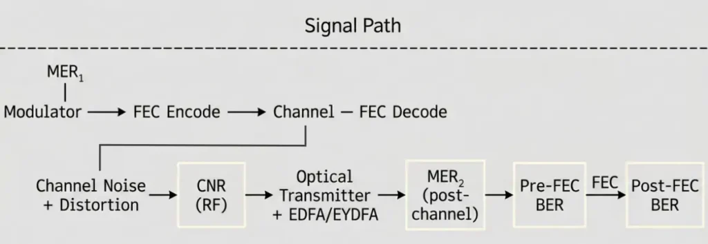
]]>The post BER and MER Explained: The Definitive Guide to Digital Signal Quality Metrics appeared first on Premlink - Homepage.
]]>1. Why BER and MER Matter
Every digital transmission system has one job: deliver bits from point A to point B without errors. In practice, noise, distortion, and impairments corrupt the signal. The question is always the same — how much corruption is too much?
Two metrics answer that question from different angles:
| Metric | What It Measures | Units | Typical Range |
|---|---|---|---|
| BER | Ratio of errored bits to total transmitted bits | Dimensionless (10−x) | 10−3 to 10−12 |
| MER | Ratio of ideal signal power to error-vector power | dB | 15 dB to 40+ dB |
BER is a result metric — it tells you the outcome after all impairments have done their damage. MER is a process metric — it tells you how much margin you have before that damage becomes catastrophic. Understanding both, and the relationship between them, is essential for anyone designing, deploying, or troubleshooting digital transmission systems.
2. BER (Bit Error Rate): Definition and Formula
2.1 Definition
Bit Error Rate (BER) is the ratio of incorrectly received bits to the total number of transmitted bits over a given observation interval. It is the most fundamental measure of digital link quality.
“BER is a measure of the number of bits received in error, specifically, the number of errored bits divided by the total number of transmitted bits.” — CableLabs, DOCSIS Radio Frequency Interface Specification
2.2 Formula
Where:
- = number of errored bits
- = total number of transmitted bits
BER is typically expressed in scientific notation as 10−x. For example:
- BER = 10−9 → on average, 1 bit error per 1,000,000,000 bits transmitted
- BER = 10−6 → on average, 1 bit error per 1,000,000 bits transmitted
- BER = 10−3 → 1 error per 1,000 bits (unacceptable for most systems)
2.3 Industry-Standard BER Thresholds
Different applications tolerate different BER levels. The following are well-established targets from ITU-T and cable industry standards:
| Application | Target BER | Standard Reference |
|---|---|---|
| Cable TV (QAM, post-FEC) | 10−8 to 10−11 | ITU-T J.83 |
| Satellite DVB-S2 (post-FEC) | 10−7 to 10−11 | ETSI EN 302 307 |
| Fiber optic (ITU-T G.652) | 10−12 (per span) | ITU-T G.957 |
| LTE/5G (data channel) | 10−5 (pre-FEC) | 3GPP TS 36.211 |
| DOCSIS 3.1 (post-FEC) | 10−8 | CableLabs CM-SP-PHYv3.1 |
A BER of 10−9 is often called the “QoS threshold” in cable systems — below this, subscribers see no visible artifacts. Above 10−6, picture quality degrades noticeably; above 10−3, the link is effectively broken.
3. MER (Modulation Error Ratio): Definition and Formula
3.1 Definition
Modulation Error Ratio (MER) is the ratio of the average power of the ideal constellation symbol to the average power of the error vector, expressed in decibels. It quantifies the aggregate impact of all impairments — noise, phase noise, amplitude imbalances, compression, and inter-symbol interference — on a modulated carrier.
“MER is to QAM signals what CNR is to analog signals — a single-number summary of signal quality, but one that captures both noise and distortion.”
3.2 Formula
Where:
- = ideal (reference) in-phase and quadrature coordinates of the j-th symbol
- = error vector components (difference between received and ideal symbol position)
- = total number of symbols measured
In the constellation diagram, this translates to:
- Numerator → Average Symbol Magnitude (the distance from origin to the ideal symbol point)
- Denominator → RMS Error Magnitude (the scatter of received symbols around their ideal positions)
3.3 MER vs. CNR: A Critical Distinction
| Aspect | CNR | MER |
|---|---|---|
| What it captures | Noise only | Noise + distortion + all impairments |
| Measurement domain | RF spectrum (power in carrier vs. noise floor) | Constellation (symbol deviations) |
| Applicable to | Any carrier (analog or digital) | QAM / QPSK modulated signals only |
| Typical relationship | MER ≤ CNR | MER is always less than or equal to CNR |
MER is always ≤ CNR because CNR measures only additive noise, while MER includes noise plus all distortion products. A system with excellent CNR but poor MER likely suffers from non-linear distortion (compression, intermodulation) or phase noise — problems CNR alone cannot detect.
3.4 MER Minimum Thresholds (Post-FEC Operational)
These are widely accepted minimum MER values for error-free reception in cable networks:
| Modulation | Minimum MER (dB) | Recommended MER (dB) | Source |
|---|---|---|---|
| QPSK | ~8–10 dB | ≥ 12 dB | ETSI TR 101 290 |
| 16-QAM | ~15–16 dB | ≥ 20 dB | ITU-T J.83 |
| 64-QAM | ~23–24 dB | ≥ 28 dB | CableLabs DOCSIS |
| 256-QAM | ~28–30 dB | ≥ 34 dB | SCTE 40 |
| 1024-QAM | ~34–36 dB | ≥ 40 dB | DOCSIS 3.1 |
| 4096-QAM | ~40–42 dB | ≥ 46 dB | DOCSIS 3.1 (full spectrum) |
Below the minimum MER, the decoder enters the “cliff effect” — signal quality drops off sharply rather than degrading gracefully. A 1–2 dB drop in MER near the threshold can mean the difference between perfect reception and total failure.
4. CNR and Its Relationship to BER
4.1 The Fundamental Trade-off: Modulation Order vs. Noise Tolerance
Higher-order QAM modulation (e.g., 256-QAM vs. QPSK) increases data throughput because each symbol carries more bits. However, this comes at a cost: the amplitude levels are spaced more closely together, making them more susceptible to noise.
| Modulation | Bits per Symbol | Relative Amplitude Spacing | CNR Sensitivity |
|---|---|---|---|
| QPSK | 2 | Widest | Lowest |
| 16-QAM | 4 | Wide | Low |
| 64-QAM | 6 | Moderate | Moderate |
| 256-QAM | 8 | Narrow | High |
| 1024-QAM | 10 | Very narrow | Very high |
| 4096-QAM | 12 | Extremely narrow | Extremely high |
4.2 CNR vs. BER: The Curves
The relationship between CNR and BER follows a characteristic family of “waterfall curves” — one for each modulation order. Based on the well-established theoretical and measured data consistent with ITU-T and CableLabs references:
Approximate CNR required for BER = 10−4 (pre-FEC):
| Modulation | Required CNR (dB) |
|---|---|
| QPSK | ~5–6 dB |
| 16-QAM | ~10–11 dB |
| 64-QAM | ~16–17 dB |
| 256-QAM | ~22–23 dB |
Approximate CNR required for BER = 10−9 (near post-FEC QoS):
| Modulation | Required CNR (dB) |
|---|---|
| QPSK | ~9–10 dB |
| 16-QAM | ~14–15 dB |
| 64-QAM | ~21–22 dB |
| 256-QAM | ~27–28 dB |
Each doubling of the modulation order (in terms of bits per symbol) typically requires approximately 5–6 dB more CNR to maintain the same BER. This is one of the most important design rules in digital transmission engineering.
4.3 Practical Implication
If your 64-QAM channel measures CNR = 25 dB, you have roughly 3–4 dB of margin above the 10−9 threshold. If you upgrade to 256-QAM to gain 33% more throughput, you need at least 28 dB CNR — meaning your margin drops to zero or negative. Without improving the link budget, the upgrade will fail.
 Optical Link Budget Matters
When the RF-to-optical conversion in the headend introduces additional noise or distortion, the CNR delivered to the receiver is degraded before the signal even reaches the coaxial distribution plant. This is why optical transmitter quality and EDFA noise figure are critical — every dB of noise added in the optical domain directly reduces the CNR available at the receiver. A low-noise optical transmitter with NPR ≥ 52 dB preserves your CNR budget and makes higher-order QAM upgrades feasible.
5. FEC (Forward Error Correction): The Safety Net
5.1 Definition
Forward Error Correction (FEC) is a technique that adds redundant bits to the transmitted data stream so that the receiver can detect and correct bit errors without requiring retransmission.
“FEC is a procedural technique used to identify and correct bit errors occurring in digital transmission. It is complex and processor-intensive, but essential for preventing bit errors that cannot be entirely eliminated from resulting in erroneous data or degraded picture quality.”
5.2 How FEC Works
FEC encoders add parity/check bits to the payload before transmission. Common FEC schemes in cable and satellite:
| System | FEC Code | Code Rate | Correction Capability |
|---|---|---|---|
| DVB-C (ITU-T J.83A/C) | Reed-Solomon (204, 188) | ~0.92 | Up to 8 byte errors per RS block |
| DOCSIS 1.0–3.0 | Reed-Solomon + interleaver | Variable | Corrects burst errors up to ~70 µs |
| DVB-S2 | LDPC + BCH | 1/4 to 9/10 | Near-Shannon-limit performance |
| DOCSIS 3.1 | LDPC + BCH | Variable | Operates within 0.8 dB of Shannon limit |
5.3 Pre-FEC BER vs. Post-FEC BER
This distinction is critical:
- Pre-FEC BER (also called “correctable BER”): The raw error rate before FEC decoding. Values like 10−4 to 10−6 are common and expected.
- Post-FEC BER (also called “uncorrectable BER”): The residual error rate after FEC decoding. For acceptable QoS, this should be essentially zero (better than 10−11).
If post-FEC BER is non-zero, it means the FEC has been overwhelmed — the incoming error rate exceeds its correction capacity. This is a red alert condition. In cable systems, a non-zero post-FEC BER directly correlates with visible pixelation, freezing, or audio dropouts.
5.4 Coding Gain
FEC provides a coding gain — the reduction in required CNR to achieve the same post-FEC BER:
| FEC Scheme | Typical Coding Gain (dB) |
|---|---|
| Reed-Solomon (204, 188) | ~2–3 dB |
| Concatenated RS + convolutional | ~5–6 dB |
| LDPC (DVB-S2) | ~8–10 dB |
| LDPC + BCH (DOCSIS 3.1) | ~9–11 dB |
This coding gain is not “free” — it costs bandwidth. A code rate of 3/4 means 25% of the transmitted bits are overhead. But in most real-world systems, the 6–10 dB coding gain is worth far more than the bandwidth penalty.
6. NPR (Noise Power Ratio): Testing Wideband QAM Systems
6.1 Definition
Noise Power Ratio (NPR) is a measurement technique used to determine the signal-to-noise performance of analog devices — amplifiers, optical transmitters, EDFAs, and EYDFAs — when loaded with multiple QAM or QPSK carriers.
Because the combined spectrum of many QAM signals closely resembles Gaussian noise, NPR testing substitutes a broadband noise source for the actual QAM signals. A narrow notch (typically 4 MHz wide) is cut into the noise, and the depth of that notch after passing through the device under test indicates the noise and distortion contributed by the device.
“NPR is sometimes referred to as a ‘notch noise test.'”
6.2 The NPR Curve
The characteristic NPR curve reveals three distinct operating regions:
| Region | Drive Level | Behavior | Dominant Mechanism |
|---|---|---|---|
| 1. System noise limited | Low | Notch depth increases 1 dB per 1 dB increase in drive | Thermal noise, shot noise dominate |
| 2. Linear operating region | Medium | Peak NPR — maximum dynamic range | Best balance: signal above noise floor, below compression |
| 3. Compression limited | High | Notch depth decreases ~5 dB per 1 dB increase in drive | Noise-like intermodulation distortion fills the notch |
The peak of the NPR curve represents the optimal operating point — the drive level at which the device delivers the best possible CNR to the loaded QAM signals.
6.3 Practical NPR Targets
For cable distribution amplifiers and optical transmission equipment carrying 64-QAM and 256-QAM:
| Device Type | Typical Peak NPR (dB) |
|---|---|
| Push-pull amplifier | 38–42 dB |
| Power-doubling amplifier | 42–46 dB |
| GaAs hybrid amplifier | 44–48 dB |
| 1550 nm optical transmitter | 50–55 dB |
| EDFA (Er-Doped Fiber Amplifier) | 52–58 dB |
| EYDFA (Er/Yb-Doped Fiber Amplifier) | 50–55 dB |
 Product Spotlight: Optical Transmitters and Amplifiers for QAM Distribution
When qualifying an optical transmitter, EDFA, or EYDFA for QAM-loaded cable or FTTH distribution, NPR is the single most important specification. Here is what to look for:
- Optical Transmitter: NPR ≥ 52 dB at rated optical output. This ensures the transmitter’s noise and distortion contribution is at least 20 dB below the QAM signal level, preserving MER for 256-QAM and beyond.
- EDFA: Noise figure ≤ 5.0 dB; NPR ≥ 54 dB at operating gain. Low NF is critical because EDFA noise is additive — once added, it cannot be removed downstream. For cascaded EDFA architectures, each stage’s NF directly subtracts from the system CNR budget.
- EYDFA: For extended-reach applications requiring output power up to 27 dBm, choose EYDFA with NF ≤ 5.5 dB and NPR ≥ 50 dB. EYDFA’s higher output power enables longer spans, but the slightly higher NF means it should be placed after a pre-amplifier EDFA in the link, not as the first amplifier stage.
Rule of thumb: in a headend-to-node optical link, the combined NPR of the optical transmitter + EDFA chain must exceed the end-of-line MER requirement by at least 6 dB to account for coaxial distribution losses.
An NPR below 30 dB at the operating point means the device is adding too much noise and distortion for reliable 256-QAM operation.
7. The Cliff Effect: Why MER Is Your Early Warning System
7.1 What Is the Cliff Effect?
In QAM systems, signal quality does not degrade linearly. There is a threshold region where a very small change in CNR or MER produces a dramatic change in BER. This is the cliff effect — named because the BER curve resembles a cliff edge.
Example for 64-QAM:
- At MER = 28 dB → BER ≈ 10−12 (effectively zero errors)
- At MER = 24 dB → BER ≈ 10−8 (still acceptable post-FEC)
- At MER = 23 dB → BER ≈ 10−6 (pre-FEC; FEC working hard)
- At MER = 21 dB → BER ≈ 10−3 (FEC overwhelmed — service failure)
A 2 dB drop near the threshold can be the difference between flawless operation and total outage.
7.2 Why MER Gives You Early Warning
Because MER is a continuous, high-resolution measurement, it can detect degradation before it shows up as uncorrectable errors. A monitoring system that tracks MER trends can alert operators when:
- MER drops below the recommended threshold (yellow alert)
- MER drops below the minimum threshold (red alert — immediate action required)
- MER is trending downward over days/weeks (preventive maintenance needed)
BER, by contrast, provides only a binary view: errors are either present or not. Once post-FEC BER goes non-zero, it is often too late for preventive action.
 Optical Amplifier Impact on the Cliff Effect
In an optical fiber distribution system, the EDFA noise figure directly determines how close you operate to the cliff edge. An EDFA with NF = 4.5 dB vs. NF = 6.0 dB gives you an extra 1.5 dB of CNR margin — which, near the cliff edge for 256-QAM, can be the difference between stable operation and intermittent failures. When selecting an EDFA or EYDFA, prioritize noise figure as the first specification — output power can always be adjusted with attenuation; noise cannot be removed once added.
8. Real-World Application: Cable Headend and Optical Distribution
8.1 Headend Quality Targets
| Parameter | Target | Measurement Point |
|---|---|---|
| MER (64-QAM) | ≥ 34 dB | QAM modulator output |
| MER (256-QAM) | ≥ 38 dB | QAM modulator output |
| Pre-FEC BER | < 10−9 | QAM modulator output |
| Post-FEC BER | 0 | QAM modulator output |
| CNR | ≥ 35 dB (64-QAM), ≥ 41 dB (256-QAM) | At first amplifier |
8.2 End-of-Line (EOL) Minimums
Per SCTE and CableLabs specifications:
| Parameter | Minimum (64-QAM) | Minimum (256-QAM) |
|---|---|---|
| MER | 23 dB | 28 dB |
| CNR | 23 dB | 28 dB |
| Post-FEC BER | 0 | 0 |
8.3 Optical Distribution Link Budget
In a typical cable headend-to-node architecture, the optical link is often the dominant contributor to CNR degradation. The key components and their impact on signal quality:
| Link Component | Key Spec for CNR/MER | Typical Value |
|---|---|---|
| 1550 nm Optical Transmitter | NPR at rated output | ≥ 52 dB |
| EDFA (trunk amplifier) | Noise Figure | ≤ 5.0 dB |
| EYDFA (extended reach) | Noise Figure + output power | NF ≤ 5.5 dB, Pout up to 27 dBm |
| Fiber attenuation | Loss per km at 1550 nm | ~0.25 dB/km (G.652.D) |
| Optical receiver | Input power range for rated CNR | −2 to +2 dBm |
Choosing the Right Optical Transmitter and Optical Amplifier
For a typical headend serving 256-QAM channels, the optical transmission chain must deliver end-of-line MER ≥ 28 dB. Here is a practical selection guide:
- Short-range (<20 km): A high-quality 1550 nm optical transmitter with NPR ≥ 52 dB may be sufficient without an in-line amplifier.
- Medium-range (20–60 km): Add an EDFA with NF ≤ 5.0 dB after the transmitter to boost signal while maintaining CNR. Choose output power 13–17 dBm for single-node distribution.
- Long-range (>60 km): Use a cascaded architecture: optical transmitter → EDFA (pre-amp) → fiber span → EYDFA (booster) → fiber span → optical receiver. The EYDFA provides the high output power (up to 27 dBm) needed for long spans, while the EDFA pre-amp keeps the noise figure low.
Always verify the combined NPR of transmitter + amplifier chain exceeds your MER target by ≥ 6 dB.
8.4 Common Failure Modes and Their MER Signatures
| Failure Mode | MER Impact | Constellation Signature |
|---|---|---|
| Thermal noise | Uniform degradation | Symmetric cloud expansion |
| Phase noise | Moderate degradation | Circular smearing |
| Amplitude compression | Selective degradation | Outer constellation points compressed inward |
| Impulse noise | Intermittent MER drops | Random bursts of scattered points |
| Co-channel interference | Pattern-specific degradation | Rotation or offset of constellation |
| Micro-reflections | Moderate degradation | Ghosting / secondary clusters |
| EDFA gain compression | Selective, load-dependent | Outer points compressed; NPR curve entering compression region |
| Optical transmitter CSO/CTB | Diagonal pattern distortion | Diagonal streaks in constellation |
9. Summary: BER, MER, CNR, FEC, and NPR — How They Fit Together
NPR validates the channel equipment (amplifiers, optical transmitters, EDFAs, EYDFAs) under realistic QAM loading conditions — ensuring the channel delivers adequate CNR/MER before signals even reach the receiver.
FAQ
Q1: What is the difference between BER and MER?
BER measures the outcome — how many bits are wrong after all impairments. MER measures the process — how much the received constellation deviates from ideal, before any bit decisions are made. MER is a continuous metric (in dB) that provides early warning of degradation; BER is a discrete metric (10−x) that reports damage after it occurs. In practice, you need both: MER for monitoring and prevention, BER for compliance verification.
Q2: What is a good MER value for 256-QAM?
For 256-QAM in cable systems, the minimum MER for error-free operation is approximately 28–30 dB (per SCTE 40 and CableLabs DOCSIS specifications). However, a recommended operational target of ≥ 34 dB provides adequate margin against the cliff effect. Below 28 dB, post-FEC BER will likely become non-zero, resulting in visible service impairments.
Q3: Why does higher-order QAM require more CNR?
Higher-order QAM (e.g., 256-QAM vs. 64-QAM) packs more bits per symbol by using more amplitude levels, which are spaced closer together. Closer spacing means smaller noise margins — a given noise amplitude is more likely to push a received symbol across a decision boundary. Approximately, each additional bit per symbol requires ~3 dB more CNR to maintain the same BER, which translates to ~5–6 dB more CNR per doubling of modulation order.
Q4: What does post-FEC BER ≠ 0 mean?
A non-zero post-FEC BER means the FEC decoder has been overwhelmed — the incoming pre-FEC error rate exceeds the correction capacity of the FEC code. This is a critical fault condition. In cable TV, it directly causes visible pixelation, frame freezes, and audio dropouts. In data networks, it triggers retransmissions and throughput collapse. Immediate troubleshooting is required: check CNR, MER, and all signal path components — including the optical transmitter and EDFA chain.
Q5: How is NPR used to qualify optical transmitters for QAM signals?
NPR testing loads the optical transmitter with broadband noise (simulating dozens of QAM carriers) and measures how deep a notch remains after passing through the device. The peak NPR value indicates the maximum achievable CNR under realistic loading. For 256-QAM cable systems, optical transmitters typically need NPR ≥ 50 dB at the operating point to deliver adequate end-of-line performance. EDFAs used in the same link should have NPR ≥ 52 dB and NF ≤ 5.0 dB.
Q6: Can MER be better than CNR?
No. MER is always less than or equal to CNR (MER ≤ CNR). CNR measures only additive noise power relative to the carrier. MER includes noise plus all distortion products (compression, intermodulation, phase noise, micro-reflections). If MER = CNR, it means the system is truly noise-limited with no significant distortion — an ideal but rarely achieved condition. In most real systems, MER is 2–6 dB below CNR due to distortion contributions from the optical transmitter, EDFA, and RF amplifiers.
References
- ITU-T Recommendation J.83, Digital multi-programme systems for television, sound and data services for cable distribution
- CableLabs, DOCSIS 3.1 Physical Layer Specification (CM-SP-PHYv3.1)
- ETSI EN 302 307, Digital Video Broadcasting (DVB); Second generation framing structure, channel coding and modulation systems for Broadcasting, Interactive Services, News Gathering and other broadband satellite applications (DVB-S2)
- SCTE 40, Digital Cable Network Interface Standard
- ETSI TR 101 290, Digital Video Broadcasting (DVB); Measurement guidelines for DVB systems
- ITU-T G.957, Optical interfaces for equipments and systems relating to the synchronous digital hierarchy
- 3GPP TS 36.211, Evolved Universal Terrestrial Radio Access (E-UTRA); Physical channels and modulation
- Broadcom, AN-3577: MER Measurement Guide for QAM Systems (Application Note)
- Cisco, Digital Signal Quality: BER, MER, and CNR (White Paper)
- Acterna / JDSU, Digital Cable TV: BER, MER, and Constellation Analysis (Technical Reference)
The post BER and MER Explained: The Definitive Guide to Digital Signal Quality Metrics appeared first on Premlink - Homepage.
]]>The post Optimizing CTB and CSO Distortion in HFC Networks: The Ultimate CATV Link Budget Guide appeared first on Premlink - Homepage.
]]>The Physics of Non-Linearity: What Drives CTB, XM, and CSO?
When multiple RF carriers pass through non-linear active components—such as the laser diodes in a CATV transmitter, the erbium-doped fiber inside an EDFA, or the photodiode within an optical receiver—they corporate to generate unwanted harmonic frequencies at specified intervals. These intermodulations degrade the clear spectral threshold of the transmission plant.
1. Composite Second Order (CSO) Distortion
CSO distortion is caused by the combination of two frequencies, resulting in sum and difference beats clustering around the visual carrier. This behavior shifts linearly on a power basis. In a typical channel allocation plan, these secondary harmonic allocations scale systematically across cascading active networks. Consequently, tracking these secondary tracking profiles is an essential step when assessing cumulative CTB and CSO Distortion behavior across a multi-stage active network.
2. Composite Triple Beat (CTB) Distortion
CTB is defined as the sum of the resultant third-order beats produced by all combinations of three frequencies that occur exactly within a specified channel frequency band. In multi-channel systems utilizing push-pull configuration architectures, CTB acts as the primary limiting performance factor.
3. Cross Modulation (XM) Distortion
XM distortion manifests when the modulation from one independent RF carrier is imposed onto another adjacent carrier within the plant. The mathematical addition properties of XM match those of CTB, as both scale exponentially on a voltage basis across active transmission systems. Because XM scales alongside third-order products, minimizing it goes hand-in-hand with deploying hardware optimized to compress global CTB and CSO Distortion margins.
Mathematical Calculations for Active Cascades
To evaluate how these non-linearities accumulate as signals pass through multiple RF amplifier stations or cascading active hardware nodes, network designers must utilize strict logarithmic summation formulas. Accurate link modeling prevents unpredictable compounding of CTB and CSO Distortion metrics at the end of a long-haul coaxial run.
1. Composite Triple Beat (CTB) Cascading Ratios
Because CTB builds up on a voltage basis, cascading identical or dissimilar nodes expands the overall distortion layout exponentially.
To add similar CTB ratios:
To add dissimilar CTB ratios:
Where:
• CTB0, CTBn = CTB (dB) of a Single Amplifier (n = 1, 2, 3, …N)
• CTBS = System CTB (dB)
• N = Number of amplifiers in cascade
Important Rules of Thumb:
• Doubling the number of amplifiers with identical CTB ratios degrades the total system CTB by exactly 6dB.
• Reducing the amplifier output level by just 1dB improves the system CTB by approximately 2dB.
2. Cross Modulation (XM) Cascading Ratios
Since XM also adds on a strict voltage basis across multi-stage active networks, its calculations mirror those of third-order triple beat distortions.
To add similar XM ratios:
To add dissimilar XM ratios:
Where:
• XM0, XMn = XM (dB) of a Single Amplifier (n = 1, 2, 3, …N)
• XMS = System XM (dB)
• N = Number of amplifiers in cascade
• Doubling the cascade count with identical XM metrics drops performance by 6dB. Reducing system output by 1dB yields a 2dB optimization margin.
3. Composite Second Order (CSO) Cascading Ratios
Unlike third-order anomalies, secondary intermodulation distortions add strictly on a power basis rather than a voltage basis, scaling down the accumulation profile curve.
To add similar CSO ratios:
To add dissimilar CSO figures:
Where:
• CSO0, CSOn = CSO (dB) of a Single Amplifier (n = 1, 2, 3, …N)
• CSOS = System CSO (dB)
• N = Number of amplifiers in cascade
Important Power-Basis Rules:
• Every time you double a cascade of similar amplifiers, system CSO degrades by 3dB.
• Reducing amplifier output specifications by 1dB improves system CSO performance margins by exactly 1dB.
Graphical Estimation of Combined Distortion Values
When engineering mixed active networks with differing noise profiles, technicians can calculate spatial adjustments manually or leverage specialized subtraction factoring charts. To graphically isolate combined performance margins between two active segments:
- Calculate the exact operational level or CNR difference between the two target active units.
- Locate the corresponding differential point horizontally along the baseline axis of the combination curve graph.
- Identify the intersecting vertical vertical subtraction factor intersection metric.
- Subtract that derived subtraction value from the lowest individual hardware baseline score to yield your clean, aggregate system value.
Critical Link Parameters for Multi-Channel CATV Systems
To design an HFC infrastructure that suppresses CTB and CSO Distortion below acceptable thresholds (typically ≥ 65dBc for analog or ≥ 50dBc for digital networks), engineers must evaluate the hardware metrics across the entire lightpath.
| Network Parameter | Typical Target Level | Primary Hardware Constraint | Impact on Picture Quality |
|---|---|---|---|
| CNR (Carrier-to-Noise) | ≥ 51 dB (Analog) / ≥ 38 dB (Digital) | Optical Input Power & Noise Figure | Snowy background, pixelation, or screen freeze |
| CSO Margin | ≥ 65 dBc (Full Channel Load) | Laser Chirp & Photodiode Symmetry | Diagonal herringbone lines and color shifting |
| CTB Margin | ≥ 65 dBc (Full Channel Load) | RF Drive Levels & Amplifier Linearity | Severe ghosting, loss of contrast, fuzzy edges |
Mitigating Intermodulation: The Premlink Hardware Solution
At Premlink, our entire engineering philosophy revolves around suppressing CTB and CSO Distortion while optimizing high-power distribution over deep fiber architectures.
1. Headend Precision with Low-Chirp EDFA Architecture
Every amplification stage introduces optical non-linearities through Self-Phase Modulation (SPM). Premlink’s high-power 1550nm PON EDFA series utilizes premium Er-Yb co-doped fibers and advanced internal microprocessors to maintain a strictly flat gain profile. By capping the optical noise figure at an ultra-low ≤ 4.5dB or 5.0dB, our EDFAs deliver massive optical budgets without pushing the fiber core into thresholds that cause severe CTB and CSO Distortion expansion.
2. High-Linearity down to the Subscriber Optical Receiver
The conversion of light back into RF energy at the home is a notorious bottleneck for harmonic generation. Premlink’s FTTH Optical Receivers utilize highly symmetrical PIN photodiodes paired with specialized GaAs push-pull amplifier modules. This integration ensures that even at fluctuating optical input powers (from −10dBm up to +2dBm), the internal circuitry automatically compensates for slope and tilt, keeping CTB and CSO Distortion firmly within carrier-grade tolerances.
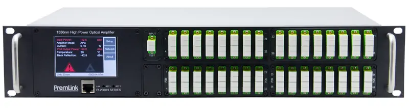
By treating the HFC network as a cohesive, closed-loop transmission link, Premlink enables ISPs to scale their multi-play services without sacrificing analog tier premium quality or digital channel data throughput.
Expert FAQ: Solving CTB and CSO Distortion Technical Bottlenecks
Q: Why does increasing the channel count make CTB and CSO Distortion significantly worse?
A: CSO increases linearly with the number of channels, but CTB grows exponentially on a voltage basis. As you add more carriers, the total composite RF voltage driving the internal laser or amplifier components pushes the linear threshold curves to saturation bounds, multiplying third-order harmonic development.
Q: How do Premlink’s hot-swappable dual power supplies protect signal distortion metrics?
A: Inconsistent voltage input creates sub-frequency ripples that directly alter amplifier bias profiles. Premlink’s carrier-grade dual power components provide flat, ripple-free current, entirely eliminating auxiliary voltage fluctuation anomalies from shifting your composite beat margins.
Q: Can adjusting the optical input power at the node improve my CSO scores?
A: Absolutely. If input margins push higher than +2dBm, physical photodiode saturation introduces immediate second-order harmonic drops. Utilizing internal attenuation fields ensures active chips remain inside their designated sweet spot, maximizing simultaneous CNR and intermodulation protection.
The post Optimizing CTB and CSO Distortion in HFC Networks: The Ultimate CATV Link Budget Guide appeared first on Premlink - Homepage.
]]>The post 1550nm Overlay Insertion for CATV: Technical Guide appeared first on Premlink - Homepage.
]]>This is where 1550nm overlay insertion comes in. The technique uses wavelength division multiplexing to layer local programming onto the same fiber that carries the primary signal. No new fibers. No major system overhaul. Just smarter use of existing infrastructure.

The Challenge: Adding Local Content Without Disruption
Large cable operators solved redundancy years ago. They deploy dual externally modulated 1550nm transmitters at the main headend. One runs active, the other sits as backup. Fiber optic switches handle automatic failover. Their entire optical network runs on this robust setup.
Small and medium operators follow a similar model, but they share one critical limitation. Their local substations need to inject locally generated content into the network stream. This local content might include regional television broadcasts, video-on-demand signals from IPQAM devices, or community announcements.
The question becomes: how do you blend these two signal sources without destroying the quality of the main programming?
How 1550nm Overlay Insertion Works
1550nm overlay insertion relies on WDM technology. Two optical signals travel through one fiber. Each signal carries a different wavelength. The primary headend uses an externally modulated transmitter. The local substation uses a directly modulated 1550nm transmitter. This approach carries a bandwidth limit. Directly modulated lasers have nonlinear distortion issues that restrict usable modulation bandwidth. In practice, 1550nm overlay insertion supports no more than 4 analog TV channels and 40 digital channels.

A WDM coupler combines both signals at the insertion point. The combined signal travels downstream through one fiber. At the receiving end, a single optical receiver picks up both wavelengths at the same time. It converts them into RF signals that share the same coaxial cable. Viewers get both national and local programming through one connection.
This approach sounds simple. The reality involves careful engineering. Power levels must balance. Wavelengths must follow standards. RF channels cannot overlap. Get any of these wrong, and the result is interference, signal degradation, or complete service failure.
Power Balancing: The Make-or-Break Factor
Power allocation between primary and overlay signals determines everything. Field testing at industry laboratories has proven this repeatedly. Here is what happens at an optical receiver input of 0dBm total power.
Scenario 1: Equal Power Split
Many engineers assume equal power sounds fair. The math tells a different story. Each wavelength receives half the total power, or -3dBm per signal. The primary signal CNR drops by the same margin as the overlay. Its output level drops by 6dB. Subscribers see visibly degraded picture quality on the main channels. This approach fails in real deployments.
Scenario 2: Unbalanced Split
A better approach assigns more power to the primary signal. Reduce the overlay power by 6dB. The primary signal now receives -1dBm. Its CNR drops only slightly. Output level drops just 2dB.
The overlay signal receives -7dBm. Its CNR drops more noticeably. Its output level falls 12dB below the primary signal. Viewers see a significant quality gap between local and main programming. Local channels look worse than national ones. This also fails, just differently.
The Solution: Boost the Local Modulation
Engineers discovered a practical fix. Increase the modulation depth of the directly modulated transmitter by 12dB. This works because the overlay signal is narrowband. It carries far fewer channels than the primary path. Raising modulation depth on a narrowband signal has minimal impact on optical link linearity. The 12dB boost compensates for both the CNR penalty and the level penalty on the overlay path. The primary and local signals end up with similar quality metrics. Subscribers receive consistent service regardless of program origin.
Industry deployments confirm this works. The technique requires no additional equipment, just proper configuration of the existing transmitter.

Three Rules for Channel Planning
1550nm overlay insertion demands strict RF channel discipline. Violate these rules, and interference ruins the viewing experience.
Rule 1: Wavelengths must differ. The overlay transmitter wavelength must never match the primary transmitter. Always select wavelengths from the ITU wavelength grid. Standard spacing prevents optical interference between the two signals.
Rule 2: RF channels cannot overlap. Local programming must use frequencies that the main signal does not occupy. For analog television, select channels between 45 and 550MHz that sit empty. For digital services, find vacant slots between 550 and 750MHz.
Rule 3: Minimize impact on primary service. Every design decision must consider the effect on the main programming. Local insertion should be transparent to existing subscribers. Their experience remains unchanged.

Distance Limitations: What 10km Really Means
Directly modulated lasers behave differently from externally modulated ones. They experience chirp effects during modulation. This limits how far the signal can travel before degradation becomes unacceptable.
Field measurements show that most directly modulated 1550nm transmitters handle fiber distances up to 10 kilometers. Beyond that, chirp-induced distortions accumulate. Signal quality drops below acceptable thresholds for broadcast television.
This range suits metropolitan networks and regional distribution systems. It does not suit long-haul applications. For longer distances, operators need additional EDFA optical amplifiers or alternative system architectures.
Putting It All Together
A practical deployment combines several components. The directly modulated 1550nm transmitter generates the local program signal. WDM technology inserts it into the main fiber path. Optical amplifiers boost the combined signal for distribution. Each substation handles its own local insertion while sharing the same fiber infrastructure.
This approach gives regional operators a cost-effective path to local content delivery. They leverage existing fiber without major construction. Subscribers receive both regional and national programming. The main signal maintains its quality standards.
The technical requirements are clear. Balance the optical power correctly. Choose ITU-standard wavelengths. Plan RF channels carefully. Respect the 10km distance limit. Follow these principles, and the system delivers reliable service for years.
Frequently Asked Questions
Q: What is 1550nm overlay insertion in CATV networks?
A:1550nm overlay insertion uses wavelength division multiplexing to add local programming to existing fiber optic cable systems. A directly modulated 1550nm transmitter carries the local content while the primary signal uses a different wavelength, allowing both to share the same fiber infrastructure.
Q: How does wavelength selection affect overlay system performance?
A: Wavelength selection follows ITU grid standards to ensure adequate separation between primary and local signals. The overlay transmitter must operate at a different wavelength than the primary transmitter to prevent optical interference and maintain signal integrity throughout the transmission path.
Q: What are the RF channel planning requirements for overlay insertion?
A: Analog channels occupy 45–550MHz while digital services use 550–750MHz. Local programming must select vacant frequencies within these ranges to avoid conflicts with primary content, ensuring viewers receive clear signals on both service tiers.
Q: How far can 1550nm overlay signals travel through fiber?
A: Directly modulated 1550nm transmitters typically support fiber distances up to 10 kilometers due to chirp effects and linear attenuation. Longer distances require amplification or alternative system architectures.
Q: Why is power balancing critical in overlay system design?
A: Power balancing determines signal quality for both primary and local content. Unequal power allocation degrades carrier-to-noise ratio and output levels. Proper balance ensures viewers experience consistent quality across all available programming.
The post 1550nm Overlay Insertion for CATV: Technical Guide appeared first on Premlink - Homepage.
]]>The post 256QAM HFC Network: How to Get 33% More Capacity Without Rebuilding Your Plant appeared first on Premlink - Homepage.
]]>- The Capacity Problem and the 256QAM Answer
- What 256QAM Demands from Your Network
- Where Does CNR Actually Get Lost?
- Modulation Depth: The One Knob That Moves Everything
- EDFA Noise: Coverage Gain, CNR Pain
- Coax Amplifier Cascades: The Silent Killer
- Putting It Together: System CNR Budget
- What to Adjust First: A Prioritized Checklist
- Frequently Asked Questions
The Capacity Problem and the 256QAM Answer
Cable operators everywhere face the same squeeze. More subscribers want more bandwidth. The spectrum you have is fixed. Building new plant takes years and costs a fortune. So when a change in modulation format promises a 33% capacity increase on the exact same infrastructure, it gets attention.
Here is the math. In the 87–862MHz downstream band, you have 96 channels at 8MHz each. Running 64QAM across all of them gives you roughly 4Gbps of total throughput. Flip to 256QAM and the same channels deliver about 5.34Gbps. That is a 33% bump.
No new fiber. No spectrum reallocation. No truck roll to swap customer equipment. On paper, it looks like the easiest capacity upgrade you will ever do.
Key point: 256QAM gives you 33% more throughput in the same 87–862MHz spectrum. But it demands a higher carrier-to-noise ratio at every point in the signal chain. If your CNR is marginal at 64QAM, it will fail at 256QAM.
And that is the catch. 256QAM is not free. It needs cleaner signals, quieter amplifiers, and more careful power budgeting at every stage. Flip the modulation switch without doing the engineering work, and your error rates will spike. Customers will notice.
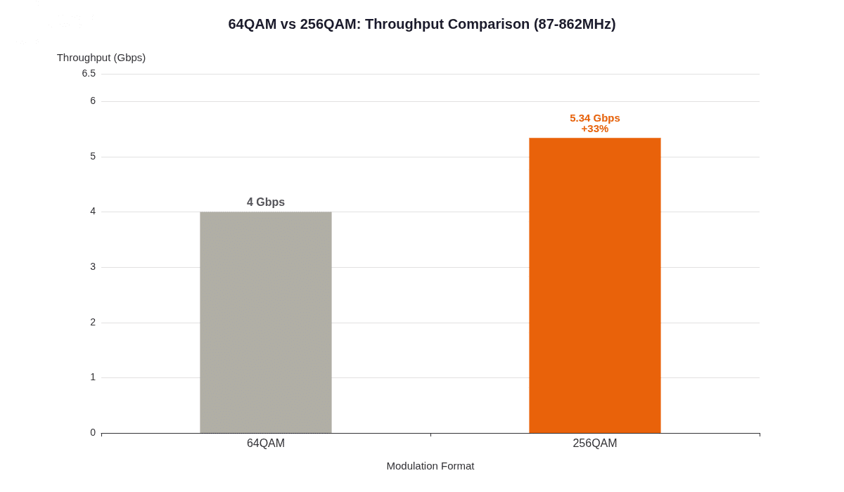
Figure 1: 64QAM vs 256QAM Capacity Comparison
At premlink, we see operators run into this over and over. They change the modulation order, errors climb, and then they spend weeks tracking down the root cause. That root cause is almost always insufficient CNR margin somewhere in the chain. This guide lays out the full picture so you can plan the move to 256QAM with eyes open.
What 256QAM Demands from Your Network
Before you touch any equipment, know the target. IEC 60728-1 defines the electrical performance your system output must meet for 256QAM. These are not suggestions. They are the line between reliable reception and customer complaints.
| Parameter | IEC 60728-1 Requirement | What It Means in Practice |
|---|---|---|
| Maximum output level | 74 dBμV | Do not exceed this at the subscriber tap |
| Minimum output level | 54 dBμV | Signal must stay above this floor |
| Minimum C/N ratio | 32 dB | This is the critical threshold for 256QAM |
| Maximum BER | 2 × 10⁻⁴ | Pre-FEC error rate limit |
| Maximum tilt | 12 dB | Level variation across the full band |
| Adjacent channel level difference | 3 dB | Keep neighboring channels close in level |
| Analog-digital level difference | 6 dB | Digital carriers run below analog |
Most of these numbers fit within what well-maintained HFC plants already deliver. The one that bites you is CNR. Going from 64QAM to 256QAM raises the minimum C/N requirement to 32dB. If your network sits at 33dB today, you have only 1dB of headroom. Temperature drifts, connectors age, and suddenly you are below the threshold.
CNR also drives BER directly. When CNR drops below spec, bit errors climb fast. Unlike analog TV where a noisy picture is still watchable, digital services either work or they do not. There is no graceful degradation with 256QAM. You meet the CNR target, or your customers see artifacts and dropouts.
Where Does CNR Actually Get Lost?
A typical 256QAM HFC network has three physical segments. Signal quality at the subscriber tap is the result of noise accumulated through all three. Understanding which segment contributes the most noise tells you where to focus your optimization effort.
Figure 2: HFC Network Signal Flow and CNR Contribution Chain
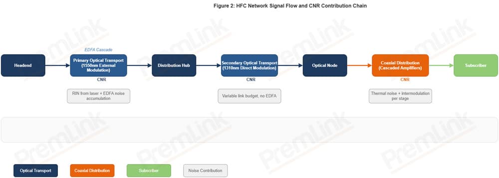
The primary optical link runs from the headend to distribution hubs on 1550nm external modulation. It often includes EDFA amplifiers to cover large areas from a single laser. Each EDFA adds noise. The more stages you cascade, the worse the accumulated relative intensity noise (RIN) gets.
The secondary optical link distributes from hubs to neighborhood optical nodes on 1310nm direct modulation. No EDFA here, but the link budget is less controlled. Fiber runs vary in length. Received optical power can swing several dB between nodes.
The coax distribution runs from the optical node to subscribers through cascaded amplifiers. Each amplifier adds thermal noise and intermodulation products. More stages mean more noise and more tilt across the band.
Here is the thing that surprises people: the noisiest segment dominates your system CNR. If your primary fiber link sits at 48dB CNR but your coax runs at 40dB, the coax sets your performance ceiling. Fixing the fiber will not help much. You have to fix the coax.
System CNR aggregates like this:
Formula (9): System CNR Aggregation
CNR₁ = input signal, CNR₂ = primary fiber, CNR₃ = secondary fiber, CNR₄ = cable network. The 10dB subtraction on CNR₃ accounts for digital carrier modulation depth being lower than analog.
That 10dB penalty on the secondary fiber term is not arbitrary. Digital carriers run at lower RF level than analog carriers. This reduces their modulation depth, which reduces their carrier power relative to noise. The formula captures that reality.
Modulation Depth: The One Knob That Moves Everything
Optical modulation depth is the single most important parameter you can adjust. It determines how much signal power you push onto the fiber, and that directly sets your CNR. Too little depth, and you waste carrier power. Too much, and you clip the laser, causing distortion that no amount of downstream filtering can fix.
The relationship starts simple. If all carriers have the same modulation depth, total modulation depth M relates to per-carrier depth mk and carrier count k like this:
Formula (2): Total Modulation Depth vs Per-Carrier Depth
M = total modulation depth, k = number of carriers, mk = per-carrier modulation depth.
Real networks run mixed analog and digital carriers, so the formula expands:
Formula (3): Mixed Analog-Digital Modulation Depth
ka = analog carrier count, ma = analog modulation depth, kd = digital carrier count, md = digital modulation depth.
Digital carriers run at lower RF level than analog. The standard practice is 10dB below analog. That level difference changes the modulation depth relationship:
Formula (4): Modulation Depth vs RF Level Difference
X = analog-digital RF level difference in dB. With X = 10dB, md ≈ 0.316 × ma.
When X = 10dB, you can simplify the mixed formula into something easier for field use:
Formula (5): Simplified Mixed Transmission (X = 10dB)
Plug in your carrier counts and target total modulation depth, and solve for ma directly.
What the Numbers Look Like in Practice
Take a typical channel plan: 93 channels in the 87–862MHz band, with 8 analog and 85 digital carriers. Here are the calculated values from industry laboratory reference data:
For 1550nm external modulation (M = 0.28):
- Analog modulation depth: 6.9%
- Digital modulation depth: 2.2%
- Analog RF level: 87.07 dBμV per channel
- Digital RF level: 77.07 dBμV per channel (10dB below analog)
For 1310nm direct modulation (M = 0.30):
- Analog modulation depth: 7.4%
- Digital modulation depth: 2.36%
- Reference RF level: 75 dBμV per channel (84 PAL D/K basis)
- Analog RF level: 82.07 dBμV per channel
- Digital RF level: 72.07 dBμV per channel
Notice the 1310nm link runs a slightly higher total modulation depth (0.30 vs 0.28). This compensates for the noise added in downstream distribution amplifiers. But it also means the 1310nm laser is closer to its clipping limit. You need to be careful not to overdrive it.
When Your Channel Count Changes
Networks do not stay static. You add or remove channels over time. When that happens, RF drive levels must change to keep total modulation depth constant. The adjustment formula is straightforward:
Formula (6): RF Level Adjustment for Channel Changes
K = number of loaded channels. Fewer channels → raise per-channel level. More channels → lower it.
If you remove channels and do not raise the remaining drive levels, you leave CNR on the table. If you add channels without reducing per-channel power, you risk clipping. Neither is good for 256QAM.
EDFA Noise: Coverage Gain, CNR Pain
EDFAs make economic sense for HFC. One optical amplifier can replace dozens of coax distribution amplifiers. Fewer active devices mean lower maintenance costs and better reliability. But EDFAs add noise, and that noise accumulates with each stage.
The core issue is relative intensity noise. Each EDFA stage adds RIN. The next stage amplifies that RIN along with the signal. The accumulated output RIN of a multi-stage EDFA cascade follows this relationship:
Formula (7): Cascaded EDFA Output RIN
E = 1.278 × 10⁻¹⁶ mJ (photon energy at 1550nm), NFk = noise figure of stage k, Pkin = input power of stage k, RINkin = input RIN of stage k.
This formula tells you something important: noise accumulation depends on each stage’s noise figure and input power. If a later stage receives degraded input power, it adds disproportionately more noise than the formula suggests on paper.
A Real Example
Consider a two-stage EDFA setup from industry laboratory measurements. The first stage output (point B) delivers 4.8dBmW. The second stage output (point C) delivers 5dBmW. Both stages have noise figures around 6.5dB. Running through the formula gives RINout ≈ -149.77 dB(Hz)⁻¹.
Without EDFA, the same 1550nm link would show RIN around -155 dB/Hz. That is a 5+ dB noise penalty just from adding two EDFA stages. In a 256QAM system where you are fighting for every decibel of CNR, that is a big deal.
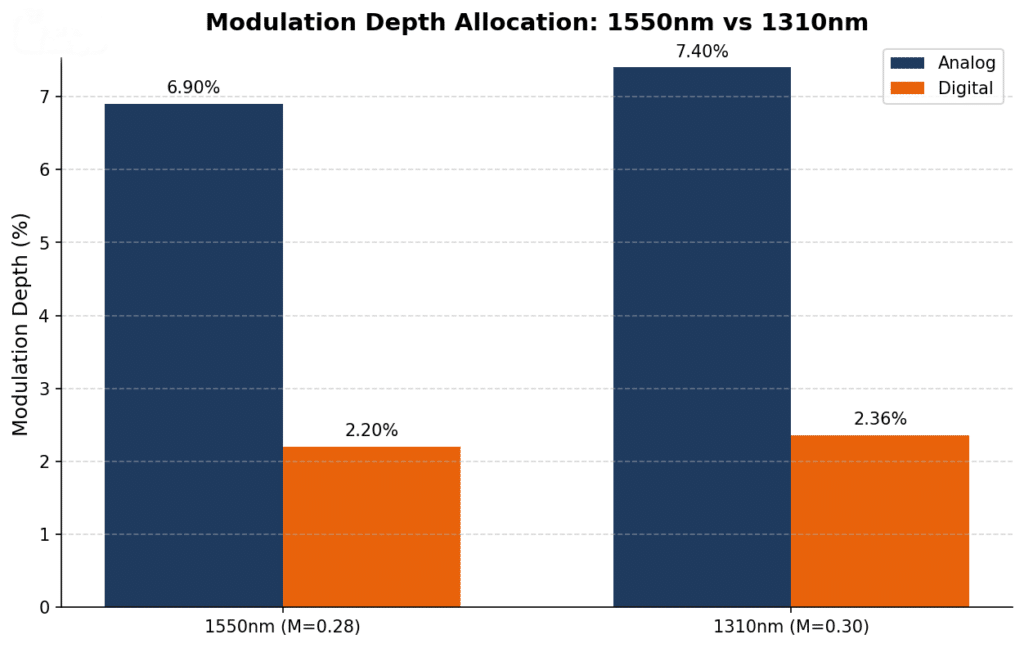
Figure 3: 1550nm CNR vs RF Drive Level (No EDFA)
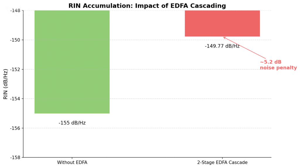
Figure 4: 1550nm CNR vs Received Optical Power (With EDFA)
Design rule: When received optical power goes above -7dBmW, EDFA noise starts dominating your noise budget. Keep EDFA input power in the 0 to -7dBmW sweet spot for 256QAM. Also, industry laboratory testing shows that 1550nm reference drive points typically sit 1dB below the CNR peak. You have room to push RF drive levels higher before clipping.
EDFA Guidelines for 256QAM
- Minimize cascade stages. Each EDFA adds noise. If you need more than two stages, rethink your fiber routing.
- Keep input power above -7dBmW. Below this, noise contributions accelerate quickly.
- Measure RIN at commissioning. Baseline measurements let you track degradation over time. RIN drift signals aging components or power instability.
- Leave 3dB of link margin. Temperature swings and connector aging will eat your margin. Plan for it.
Coax Amplifier Cascades: The Silent Killer
The coax distribution network gets less attention than fiber, but it often determines whether 256QAM works or fails. Each amplifier in a cascade adds thermal noise and intermodulation products. More stages compound both problems in ways that devastate high-order modulation.
Let us be blunt: for 256QAM, keep your amplifier cascades to four stages or fewer. This is not a guideline you can bend. Four stages match the performance of fiber-deep architectures across the full 87–862MHz band. Five stages degrade frequencies above 650MHz by 1–2dB. Six or more stages push performance into unacceptable territory.
Field reality: If your plant runs more than four amplifier stages between the optical node and the subscriber, 256QAM will not work reliably. No amount of level tweaking fixes excessive cascade depth. You need node segmentation or fiber extension.
Amplifier Noise Math
IEC specifies minimum 45dB CNR for cable networks in MDU (multi-dwelling unit) environments. The cable network CNR follows:
Formula (8): Cable Network CNR
Si = cable network input level (75 dBμV), F = amplifier noise figure (10 dB), n = number of cascade stages.
With Si = 75 dBμV and F = 10 dB, you can calculate CNR for different cascade depths:
| Cascade Stages | CNR (dB) | Meets 45dB MDU Spec? |
|---|---|---|
| 2 | 57.6 | Yes, with large margin |
| 4 | 51.6 | Yes |
| 6 | 48.6 | Yes, but tight |
| 10 | 44.6 | No — below 45dB spec |
Those numbers look like you could run 6 or even 8 stages and still hit 45dB. But CNR is only half the story. Distortion products also accumulate with cascade depth, and they hit 256QAM carriers harder than the CNR math suggests.
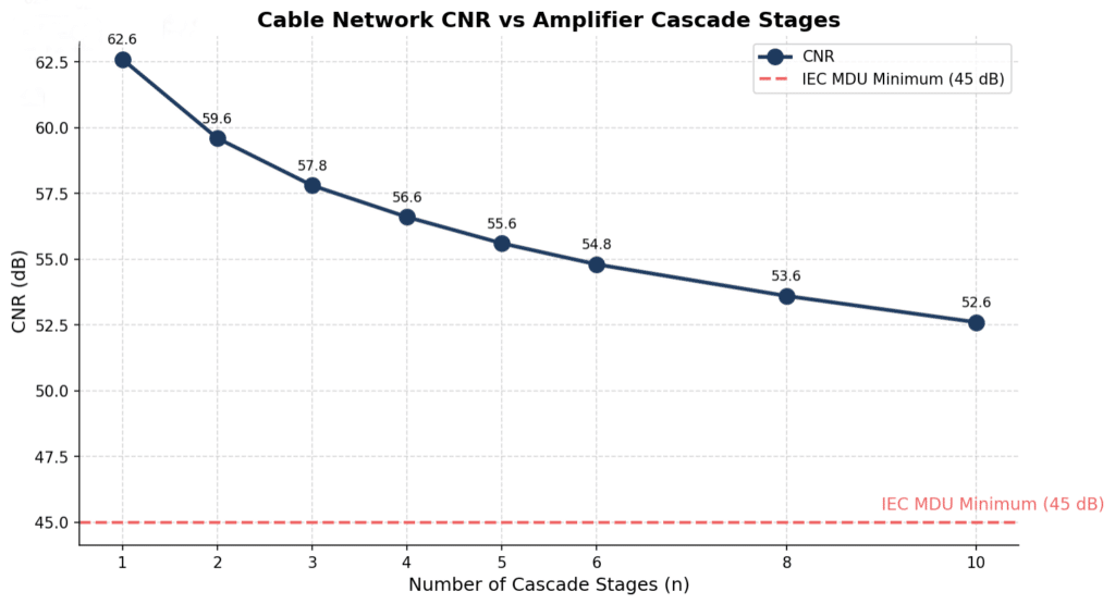
Figure 5: Frequency Response vs Amplifier Cascade Depth
Industry laboratory measurements confirm this. Four amplifier stages keep the frequency response flat across 87–862MHz. Five stages introduce 1–2dB droop above 650MHz. Six or more stages show divergent roll-off that makes 256QAM on upper channels impossible. Cable attenuation increases with frequency, and each amplifier stage adds tilt compensation error that accumulates. Passive splitters and taps make it worse because their high-frequency loss exceeds theoretical predictions.
Putting It Together: System CNR Budget
Individual segment performance does not guarantee end-to-end performance. You have to budget CNR across all segments. This is where many 256QAM deployments stumble. Engineers optimize each segment in isolation and miss the aggregate.
The IEC CNR formula for individual optical links is the foundation:
Formula (1): IEC Optical Link CNR
BN = noise bandwidth, mk = per-carrier modulation depth, R = receiver responsivity, Pr = received optical power, RIN = relative intensity noise, e = electron charge, Id0 = dark current, Ieq = equivalent input noise current.
This formula separates signal power from three noise sources: laser RIN, shot noise (from dark current and photocurrent), and receiver thermal noise. Signal power depends on modulation depth and received optical power. If either drops, CNR drops with it.
A Worked Example
Let us plug in realistic values and see what the system CNR looks like:
- Input signal CNR for analog: 50 dB
- Input signal CNR for 256QAM: 37.9 dB
- Primary fiber CNR (two-stage EDFA, 0dBmW received): ~50 dB
- Secondary fiber CNR (1310nm, -5dBmW received): ~48 dB
- Cable network CNR (4-stage cascade): ~52 dB
- Analog-digital level difference: 10 dB
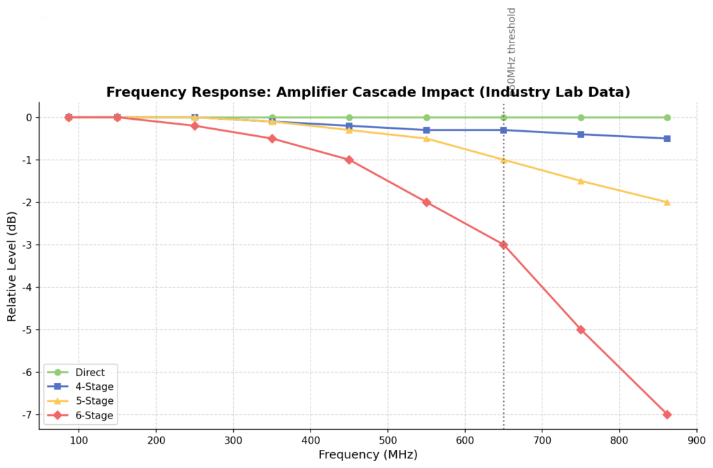
Figure 6: System Output CNR vs Secondary Fiber Received Power
Running through the system CNR aggregation formula, the result lands around 35–37dB for the digital carriers. That gives you 3–5dB of margin above the 32dB IEC minimum. Not luxurious, but workable. If any segment degrades by even 2–3dB, you lose your margin.
The key insight from this exercise: secondary fiber received optical power is the binding constraint. When it drops below -10dBmW, system CNR for 256QAM falls below the 32dB threshold. This is where you need the most careful engineering.
What to Adjust First: A Prioritized Checklist
Here is what to actually do, in order of impact and effort.
Priority 1: Primary Fiber RF Drive Levels
Your headend settings affect everything downstream. Get these right first:
- Push RF drive toward full modulation. Industry laboratory testing shows that typical 1550nm platforms run about 1dB below the CNR peak at reference settings. You have room to increase drive levels. Use it.
- Control EDFA input power to 0–3dBmW. Below -7dBmW, EDFA noise starts eating your CNR budget.
- Track RIN over time. Baseline at commissioning. RIN drift predicts failures before they affect customers.
Priority 2: Secondary Fiber Settings
This segment often gets less attention. That is a mistake:
- Do not run at the clipping limit. The 1310nm link is closer to its modulation ceiling than the 1550nm link. Leave 2–3dB of headroom to prevent digital peak clipping.
- Keep received optical power above -10dBmW. This is the hard floor. Below it, your system CNR budget fails.
- Account for variable fiber lengths. Secondary links serve different distances. Budget optical power for the longest run, not the average.
Priority 3: Coax Cascade Reduction
If your cascade exceeds four stages, no adjustment helps. You need physical changes:
- Count your amplifier stages. If you find five or more between node and subscriber, plan a segmentation project.
- Extend fiber deeper. Moving the optical node closer to subscribers eliminates cascade stages without adding cabinet equipment.
- Upgrade old amplifiers. Modern push-pull and GaAs amplifiers offer better noise figures and lower distortion than legacy modules.
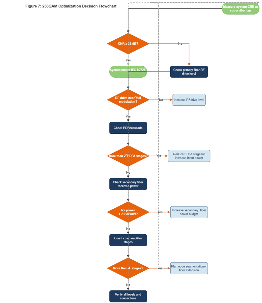
Figure 7: 256QAM Optimization Decision Flow
Priority 4: Ongoing Monitoring
Optimization is not a one-and-done activity:
- Set baselines. Measure CNR, MER, and BER at key nodes when everything is working right.
- Watch trends, not just thresholds. A 1dB CNR decline over six months predicts problems. Fix it before customers notice.
- Adjust for seasons. Laser output and fiber loss change with temperature. In extreme climates, seasonal level adjustments may be necessary.
As we emphasize at premlink.net, the difference between networks that successfully deploy 256QAM and those that struggle comes down to margin management. The 33% capacity gain is real, but it lives inside a narrow CNR window. Protect that window, and the upgrade pays for itself. Ignore it, and you spend more on troubleshooting than you saved on the modulation change.
Frequently Asked Questions
Q:How much capacity does 256QAM add over 64QAM in HFC networks?
A: In the 87–862MHz band with 96 channels of 8MHz each, 64QAM gives you about 4Gbps. 256QAM pushes that to roughly 5.34Gbps. That is a 33% gain on the same spectrum, the same fiber, the same coax.
Q: What minimum CNR does IEC 60728-1 require for 256QAM?
A: IEC 60728-1 sets the minimum carrier-to-noise ratio at 32dB for 256QAM at the system output. Other requirements include maximum output level 74dBμV, minimum output level 54dBμV, maximum tilt 12dB, adjacent channel level difference 3dB, and analog-digital level difference 6dB.
Q: Why does EDFA make CNR worse in 1550nm HFC links?
A: Each EDFA stage adds relative intensity noise (RIN). A two-stage EDFA cascade raises RIN from about -155dB/Hz to roughly -149.77dB/Hz. That 5+ dB noise penalty eats into your CNR budget. When received optical power goes above -7dBmW, EDFA noise starts dominating the total noise floor.
Q: How many coax amplifier stages can a 256QAM HFC network tolerate?
A: Keep it to four stages or fewer. Four stages match fiber-deep performance across 87–862MHz. Five stages degrade frequencies above 650MHz by 1–2dB. Six or more stages make 256QAM unreliable.
Q: What is the system-level CNR formula for HFC networks?
A:
where CNR1 through CNR4 are input signal, primary fiber, secondary fiber, and cable network CNR values. The 10dB subtraction on CNR3 accounts for the digital carrier modulation depth penalty.
Q: What optical receive power should I target for 256QAM?
A: For 1550nm links with EDFA, aim for 0 to +3dBmW. For 1310nm secondary links, stay above -10dBmW. Always leave headroom—running at the minimum leaves no room for aging, temperature swings, or fiber connector degradation.
Q: How does analog-digital level difference affect modulation depth?
A: Digital carriers run 10dB below analog carriers. The modulation depth relationship is
With X=10dB, digital modulation depth is about 31.6% of analog depth. IEC 60728-1 specifies a 6dB analog-digital level difference for 256QAM systems.
Q: Can I run 256QAM across the full 87-862MHz band on existing HFC plant?
A: Yes, but only if your CNR budget clears 32dB at every system output point. That means optimizing RF drive levels, managing EDFA cascade noise, keeping amplifier stages to four or fewer, and maintaining proper optical power budgets. It is not a software switch—it requires engineering work.
About premlink.net: This guide is part of premlink.net’s technical library for the CATV optical communications industry. Find more products, such as optical transmitter, EDFA at our products center.
The post 256QAM HFC Network: How to Get 33% More Capacity Without Rebuilding Your Plant appeared first on Premlink - Homepage.
]]>The post International TV Standards and Voltage Reference: The Ultimate Infrastructure Guide for Video Distribution appeared first on Premlink - Homepage.
]]>The Technical Pillars of Global Video Transmission
Deploying a video network in a foreign territory requires a granular approach to hardware configuration. Whether you are scaling a network in Southeast Asia or Latin America, you must harmonize three critical variables: the colour encoding system, the RF frequency channel plan, and the local power grid specifications.
1. Colour Encoding & Modulation
While the world has moved toward digital, the legacy of analogue International TV Standards still dictates the physical layer of RF distribution. NTSC (30 fps) dominates North America and parts of Asia, while PAL (25 fps) provides superior colour stability across Europe, China, and Africa. SECAM, though less common today, still influences channel spacing in specific regions. Your equipment must be transparent to these modulations to ensure zero signal degradation.
2. RF Frequency Allocations for International TV Standards
A “Channel 5” in one country is not a “Channel 5” in another. The channel frequency standards (such as B/G, D/K, or I) determine the gap between the video and audio carriers. While the digital transition is accelerating, the legacy International TV Standards still define the bandwidth filtering and signal-to-noise ratio (SNR) requirements for cable plants. For a technician, misidentifying these standards can lead to severe ghosting or signal overlap.
Deep Dive: The Non-Compatibility of NTSC, PAL, and SECAM
A fundamental challenge in global broadcasting is that NTSC, PAL, and SECAM—the three primary International TV Standards—are inherently incompatible. For example, playing an NTSC video on a native PAL system will result in scrambled synchronization or a complete loss of image. Understanding these differences is non-negotiable for manufacturers and exporters.
I. NTSC (National Television System Committee)
Established in 1952 in the USA, NTSC (often called “N-format”) operates at a frame rate of 29.97 fps with 525 scan lines. Using interlaced scanning and a 4:3 aspect ratio (720×480 resolution), it employs balanced and quadrature modulation. While it enabled color/black-and-white compatibility, its primary weakness is phase sensitivity, which causes color instability. This requires manual “tint control” on older sets. NTSC is the core of International TV Standards for North America, Canada, Mexico, Japan, South Korea, and the Philippines.
II. SECAM (Séquential Couleur Avec Mémoire)
Developed in France in 1966, SECAM (“Sequential Color with Memory”) avoids color distortion by transmitting color difference signals sequentially. It operates at 25 fps with 625 scan lines (720×576 resolution). While SECAM is highly resistant to interference and offers excellent color results, it lacks the broad compatibility of other International TV Standards. It is primarily used in Russia, France, Egypt, and French-speaking African nations.
III. PAL (Phase Alternating Line)
Introduced in 1967 in Germany, PAL (“Phase Alternating Line”) was designed to overcome NTSC’s color shifts. By reversing the phase of the color signal on every other line, PAL automatically corrects phase distortions occurring during transmission. Operating at 25 fps with 625 scan lines, PAL offers superior color accuracy and compatibility with black-and-white sets. Modern International TV Standards recognize PAL-D (China) and PAL-I (UK/Hong Kong) as its major sub-formats.
Technical Note: Film Playback on PAL vs. NTSC
Since cinema is shot at 24 fps, NTSC uses “2:3 Pull-Up” to match its 30 fps rate, maintaining original speed. However, PAL typically plays 24 fps film at 25 fps, meaning the movie plays 4% faster. To maintain synchronization, the audio pitch must be adjusted, a critical detail when configuring equipment for different International TV Standards.
Definitive A-to-Z Broadcast Standards & Power Reference Table
To assist global engineering teams, we have compiled the following exhaustive technical database. This reference aligns International TV Standards with power grid parameters, serving as a critical cross-check for anyone configuring high-density optical hardware for international export.
| Country | Format | VHF | UHF | Channel Freq. Standard | Voltage | Frequency |
|---|---|---|---|---|---|---|
| Afghanistan | PAL / SECAM | B | – | B | 220 V | 50 Hz |
| Albania | PAL | B | G | B/G | 220 V | 50 Hz |
| Algeria | PAL | B | – | B | 227‑220 V | 50 Hz |
| Angola | PAL | I | – | I | 220 V | 50 Hz |
| Andorra | PAL | B | G | B/G | 220 V | 50 Hz |
| Argentina | PAL‑N | N | – | N | 220 V | 50 Hz |
| Armenia | SECAM | D | K | D/K | 220 V | 50 Hz |
| Aruba | NTSC | M | – | M | 120 V | 60 Hz |
| Australia | PAL | B | – | B | 240‑230 V | 50 Hz |
| Austria | PAL | B | G | B/G | 220‑230 V | 50 Hz |
| Azerbaijan | SECAM | D | K | D/K | 220 V | 50 Hz |
| Bahamas | NTSC | M | – | M | 120 V | 60 Hz |
| Bahrain | PAL | B | G | B/G | 120‑230 V | 60 Hz |
| Bangladesh | PAL | B | – | B | 220 V | 50 Hz |
| Barbados | NTSC | M | – | M | 115‑120 V | 50 Hz |
| Belarus | SECAM | D | K | D/K | 220 V | 50 Hz |
| Belgium | PAL | B | H | B/H | 127‑220 V | 50 Hz |
| Belize | NTSC | M | – | M | 110 V | 60 Hz |
| Benin | SECAM | K1 | – | K1 | 220 V | 50 Hz |
| Bermuda | NTSC | M | – | M | 120 V | 60 Hz |
| Bhutan | PAL | B | – | B | 220 V | 50 Hz |
| Bolivia | NTSC | M | – | M | 115‑230 V | 50 Hz |
| Bosnia & Herzegovina | PAL | B | H | B/H | 220 V | 50 Hz |
| Botswana | SECAM | K | – | K | 230 V | 50 Hz |
| Brazil | PAL‑M | M | – | M | 110‑220 V | 60 Hz |
| Brunei | PAL | B | – | B | 230 V | 50 Hz |
| Bulgaria | SECAM | D | K | D/K | 220 V | 50 Hz |
| Burkina Faso | SECAM | K | – | K | 220 V | 50 Hz |
| Burundi | SECAM | K | – | K | 230 V | 50 Hz |
| Cambodia | NTSC / PAL | M | – | M | 110‑220 V | 50 Hz |
| Cameroon | PAL | B | G | B/G | 127‑220 V | 50 Hz |
| Canada | NTSC | M | – | M | 110‑240 V | 60 Hz |
| Chile | NTSC | M | – | M | 220 V | 50 Hz |
| China | PAL | D | – | D/K | 220 V | 50 Hz |
| Colombia | NTSC | M | – | M | 110‑220 V | 60 Hz |
| Comoros | SECAM | K | – | K | 220 V | 50 Hz |
| Congo | SECAM | K | – | K | 220 V | 50 Hz |
| Costa Rica | NTSC | M | – | M | 120 V | 60 Hz |
| Croatia | PAL | B | H | B/H | 220 V | 50 Hz |
| Cuba | NTSC | M | – | M | 110‑220 V | 60 Hz |
| Cyprus | PAL | B | G | B/G | 220 V | 50 Hz |
| Czech Republic | PAL | D | K | D/K | 220‑230 V | 50 Hz |
| Denmark | PAL | B | G | B/G | 230 V | 50 Hz |
| Djibouti | SECAM | B | – | B | 220 V | 50 Hz |
| Dominican Republic | NTSC | M | – | M | 110‑220 V | 60 Hz |
| Ecuador | NTSC | M | – | M | 110‑220 V | 60 Hz |
| Egypt | PAL | B | – | B | 220 V | 50 Hz |
| El Salvador | NTSC | M | – | M | 110‑220 V | 60 Hz |
| Estonia | PAL | B | G | B/G | 230 V | 50 Hz |
| Ethiopia | PAL | B | – | B | 220 V | 50 Hz |
| Faeroe Islands | PAL | B | G | B/G | 220 V | 50 Hz |
| Finland | PAL | B | G | B/G | 230 V | 50 Hz |
| France | SECAM | L | – | L | 230 V | 50 Hz |
| Gabon | SECAM | K1 | – | K1 | 220 V | 50 Hz |
| Gambia | PAL | I | – | I | 220‑230 V | 50 Hz |
| Germany | PAL | B | G | B/G | 230 V | 50 Hz |
| Ghana | PAL | B | – | B | 220‑230 V | 50 Hz |
| Gibraltar | PAL | B | – | B | 240 V | 50 Hz |
| Greece | SECAM (B/G) | B | G | B/G | 230 V | 50 Hz |
| Greenland | PAL | B | – | B | 220 V | 50 Hz |
| Guam | NTSC | M | – | M | 110‑120 V | 60 Hz |
| Guatemala | NTSC | M | – | M | 110‑120 V | 60 Hz |
| Guinea | SECAM | K1 | – | K1 | 220 V | 50 Hz |
| Guinea‑Bissau | SECAM | K1 | – | K1 | 220 V | 50 Hz |
| Honduras | NTSC | M | – | M | 110‑220 V | 60 Hz |
| Hong Kong | PAL | I | – | I | 220 V | 50 Hz |
| Hungary | PAL | D | K | D/K | 230 V | 50 Hz |
| Iceland | PAL | B | G | B/G | 230 V | 50 Hz |
| India | PAL | B | – | B | 230 V | 50 Hz |
| Indonesia | PAL | B | – | B | 220 V | 50 Hz |
| Iran | SECAM | B | – | B | 230 V | 50 Hz |
| Iraq | SECAM | B | – | B | 230 V | 50 Hz |
| Ireland | PAL | I | – | I | 230 V | 50 Hz |
| Israel | PAL | B | G | B/G | 230 V | 50 Hz |
| Italy | PAL | B | G | B/G | 230 V | 50 Hz |
| Jamaica | NTSC | M | – | M | 110 V | 50 Hz |
| Japan | NTSC | M | – | M | 100 V | 50/60 Hz |
| Jordan | PAL | B | G | B/G | 230 V | 50 Hz |
| Kenya | PAL | B | – | B | 240 V | 50 Hz |
| Korea, North | PAL | D | K | D/K | 220 V | 60 Hz |
| Korea, South | NTSC | M | – | M | 110‑220 V | 60 Hz |
| Kuwait | PAL | B | G | B/G | 240 V | 50 Hz |
| Latvia | PAL | B | G | B/G | 230 V | 50 Hz |
| Lebanon | SECAM | B | G | B/G | 230 V | 50 Hz |
| Libya | PAL | B | – | B | 127‑230 V | 50 Hz |
| Lithuania | PAL | B | G | B/G | 230 V | 50 Hz |
| Luxembourg | PAL / SECAM | B | G/L | B/G/L | 230 V | 50 Hz |
| Macau | PAL | I | – | I | 220 V | 50 Hz |
| Malaysia | PAL | B | – | B | 230 V | 50 Hz |
| Maldives | PAL | B | – | B | 230 V | 50 Hz |
| Malta | PAL | B | H | B/H | 230 V | 50 Hz |
| Mauritius | SECAM | – | – | – | 230 V | 50 Hz |
| Mexico | NTSC | M | – | M | 127 V | 60 Hz |
| Monaco | PAL / SECAM | G | L | G/L | 230 V | 50 Hz |
| Mongolia | SECAM | D | – | D | 220 V | 50 Hz |
| Morocco | SECAM | B | – | B | 127‑220 V | 50 Hz |
| Mozambique | PAL | I | – | I | 220 V | 50 Hz |
| Myanmar (Burma) | NTSC | M | – | M | 230 V | 50 Hz |
| Nepal | PAL | B | – | B | 230 V | 50 Hz |
| Netherlands | PAL | B | G | B/G | 230 V | 50 Hz |
| New Zealand | PAL | B | – | B | 220‑240 V | 50 Hz |
| Nicaragua | NTSC | M | – | M | 110 V | 60 Hz |
| Niger | SECAM | K | – | K | 220 V | 50 Hz |
| Nigeria | PAL | I | – | I | 240 V | 50 Hz |
| Norway | PAL | B | G | B/G | 230 V | 50 Hz |
| Oman | PAL | B | G | B/G | 240 V | 50 Hz |
| Pakistan | PAL | B | – | B | 230 V | 50 Hz |
| Panama | NTSC | M | – | M | 110‑220 V | 60 Hz |
| Paraguay | PAL‑N | N | – | N | 220 V | 50 Hz |
| Peru | NTSC | M | – | M | 220 V | 60 Hz |
| Philippines | NTSC | M | – | M | 220 V | 60 Hz |
| Poland | PAL | D | K | D/K | 230 V | 50 Hz |
| Portugal | PAL | B | G | B/G | 230 V | 50 Hz |
| Puerto Rico | NTSC | M | – | M | 110‑120 V | 60 Hz |
| Qatar | PAL | B | G | B/G | 240 V | 50 Hz |
| Romania | PAL | D | K | D/K | 230 V | 50 Hz |
| Russia | SECAM | D | K | D/K | 220 V | 50 Hz |
| Saudi Arabia | PAL / SECAM | B | G | B/G | 220 V / 127 V | 50/60 Hz |
| Senegal | SECAM | K | – | K | 230 V | 50 Hz |
| Serbia | PAL | B | G | B/G | 230 V | 50 Hz |
| Singapore | PAL | B | G | B/G | 230 V | 50 Hz |
| Slovakia | PAL | D | K | D/K | 230 V | 50 Hz |
| Slovenia | PAL | B | G | B/G | 230 V | 50 Hz |
| South Africa | PAL | I | – | I | 220‑240 V | 50 Hz |
| Spain | PAL | B | G | B/G | 230 V | 50 Hz |
| Sri Lanka | PAL | B | – | B | 230 V | 50 Hz |
| Sudan | PAL | B | – | B | 230‑240 V | 50 Hz |
| Suriname | NTSC | M | – | M | 127‑220 V | 60 Hz |
| Swaziland (Eswatini) | PAL | I | – | I | 230 V | 50 Hz |
| Sweden | PAL | B | G | B/G | 230 V | 50 Hz |
| Switzerland | PAL | B | G | B/G | 230 V | 50 Hz |
| Syria | SECAM | B | – | B | 220 V | 50 Hz |
| Taiwan | NTSC | M | – | M | 110 V | 60 Hz |
| Tanzania | PAL | I | – | I | 230 V | 50 Hz |
| Thailand | PAL | B | – | B | 220 V | 50 Hz |
| Togo | SECAM | K | – | K | 220 V | 50 Hz |
| Trinidad & Tobago | NTSC | M | – | M | 115‑230 V | 60 Hz |
| Tunisia | SECAM | B | – | B | 230 V | 50 Hz |
| Turkey | PAL | B | G | B/G | 230 V | 50 Hz |
| Uganda | PAL | B | – | B | 240 V | 50 Hz |
| Ukraine | SECAM | D | K | D/K | 220‑230 V | 50 Hz |
| United Arab Emirates | PAL | B | G | B/G | 230‑240 V | 50 Hz |
| United Kingdom | PAL | I | – | I | 230 V | 50 Hz |
| United States | NTSC | M | – | M | 110‑120 V | 60 Hz |
| Uruguay | PAL‑N | N | – | N | 220 V | 50 Hz |
| Venezuela | NTSC | M | – | M | 110‑220 V | 60 Hz |
| Vietnam | NTSC / PAL | M | – | M | 220 V | 50 Hz |
| Yemen | PAL | B | G | B/G | 220‑230 V | 50 Hz |
| Zambia | PAL | I | – | I | 230 V | 50 Hz |
| Zimbabwe | PAL | I | – | I | 220‑240 V | 50 Hz |
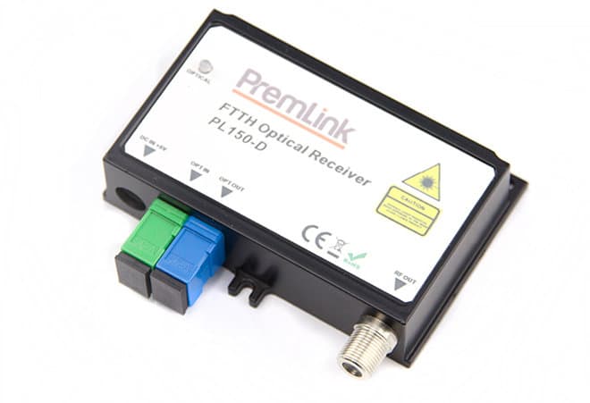
Strategic Implementation of Multi-Standard Optical Links
Navigating the fragmented landscape of International TV Standards requires a hardware ecosystem that is as flexible as it is powerful. For a network operator, the goal is “universal transparency”—a state where the transmission equipment does not care about the underlying modulation but delivers it with zero jitter. By integrating adaptive filters and wide-band amplification, Premlink ensures that your infrastructure remains compliant with all major International TV Standards without needing costly hardware swaps for each new region.
Furthermore, as digital QAM and IPTV continue to grow, maintaining backward compatibility with analogue International TV Standards is essential for customer retention in hybrid markets. Premlink’s latest EDFA and receiver series are designed with this transition in mind, providing the necessary RF headroom to support legacy carriers alongside high-density digital data streams. This dual-capability ensures that your investment in International TV Standards hardware remains relevant for the next decade of network evolution.
Beyond the Table: Scaling Your Network with Premlink
Knowing the International TV Standards is the first step; having the hardware that can adapt to them is the second. At Premlink, we design our optical transmission equipment to be globally agile. By adhering to strict International TV Standards during the R&D phase, we ensure our products exceed local performance expectations.
Optimizing the Link with FTTH Optical Receivers
The Premlink PL150D receiver is built with an agile internal filtering system that caters to the diverse International TV Standards found in our chart. Its GaAs (Gallium Arsenide) amplifier stage is optimized to provide a flat RF response across the entire frequency spectrum, ensuring that whether the channel plan follows PAL B/G or NTSC M, the subscriber enjoys premium video clarity.
The Core of Convergence: PON EDFA
To manage a network spanning various International TV Standards, a powerful and clean light source is mandatory. Premlink’s PON EDFA solutions allow for the seamless multiplexing of 1550nm video with 10G-PON data (1270/1577nm). By providing a high-power budget, our EDFAs ensure that the 1550nm carrier remains robust enough to be decoded by any local tuner, regardless of the modulation format. This versatility is why Premlink is a leader in compliant International TV Standards hardware.
Ultimately, mastering the complexities of International TV Standards allows operators to build more resilient and future-proof networks. By selecting Premlink’s standardized yet adaptable hardware, you ensure that your global deployments remain stable and cost-effective across all five continents.
Expert FAQ: Navigating Global Broadcast Challenges
Q: Can one optical receiver handle different International TV Standards?
A: Yes. High-quality receivers like the Premlink PL150D are modulation-transparent. However, the RF output level and slope should be fine-tuned based on the specific channel frequency standard (e.g., D/K vs. B/G).
Q: Why does Premlink emphasize 6KV protection for certain standards?
A: Many regions using PAL or NTSC standards are located in tropical climates. Based on our database of International TV Standards, these areas often suffer from frequent lightning. 6KV protection is a “must-have” to reduce maintenance costs.
Q: How does the power frequency (50Hz vs 60Hz) affect my EDFA?
A: While the fiber signal is unaffected, the internal power supply of the EDFA must be rated for the local frequency to ensure long-term stability according to various International TV Standards requirements.
The post International TV Standards and Voltage Reference: The Ultimate Infrastructure Guide for Video Distribution appeared first on Premlink - Homepage.
]]>